Animal Crossing: New Horizons kept me sane throughout the first Melbourne COVID lockdown. Now, in lockdown 4, it seems right that I should look back at this cheerful, relaxing game and do some data stuff. I’m going to take the Animal Crossing villagers in the Tidy Tuesday Animal Crossing dataset and combine it with survey data from the Animal Crossing Portal, giving each villager a measure of popularity. I’ll use the Google Cloud Vision API to annotate each of the villager thumbnails, and with these train a a (pretty poor) model of villager popularity.
library(tidyverse)
library(tidymodels)
library(glue)
library(httr)
library(ggimage)
library(patchwork)
library(lime)
Retrieve the villager popularity votes
The Animal Crossing Portal is a fan site that runs a monthly poll on favourite villagers. They keep historical data in publicly available Google Sheets, which makes a data scientist like me very happy.
The sheet is a list of votes, but two columns to the side tally the total votes for each villager. That leaves a lot of dangling empty rows. I’ll grab those two columns and delete the empty rows.
popularity_url <- "https://docs.google.com/spreadsheets/d/1ADak5KpVYjeSRNN4qudYERMotPkeRP5n4rN_VpOQm4Y/edit#gid=0"
googlesheets4::gs4_deauth() # disable authentication for this public sheet

popularity <- googlesheets4::read_sheet(popularity_url) %>%
    transmute( # transmute combines mutate and select
        name = Villagers,
        popularity = Tally
    ) %>%
    na.omit()
#> Reading from "April 2021 Poll Final Vote Count"
#> Range "Sheet1"
#> New names:
#> * `` -> ...7
#> * `` -> ...10

popularity %>% arrange(-popularity) %>% head()
#> # A tibble: 6 x 2
#>   name    popularity
#>   <chr>        <dbl>
#> 1 Marshal        725
#> 2 Raymond        656
#> 3 Sherb          579
#> 4 Zucker         558
#> 5 Judy           421
#> 6 Fauna          407
Retrieve the Tidy Tuesday villager data
I always come late to the Tidy Tuesday party. This is the dataset from 2020-05-05. It contains a data frame of every villager available in Animal Crossing: New Horizons (at the time), with their gender, species, and a few other attributes. It also contains a url column pointing to a thumbnail of the villager — I’ll use this later when I’m querying the Vision API.
tidy_tuesday_data <- tidytuesdayR::tt_load("2020-05-05")
#>
#>   Downloading file 1 of 4: `critic.tsv`
#>   Downloading file 2 of 4: `items.csv`
#>   Downloading file 3 of 4: `user_reviews.tsv`
#>   Downloading file 4 of 4: `villagers.csv`
tidy_tuesday_villagers <- tidy_tuesday_data$villagers
tidy_tuesday_villagers %>% head()
#> # A tibble: 6 x 11
#>   row_n id     name   gender species birthday personality song   phrase full_id
#>   <dbl> <chr>  <chr>  <chr>  <chr>   <chr>    <chr>       <chr>  <chr>  <chr>
#> 1     2 admir… Admir… male   bird    1-27     cranky      Steep… aye a… village…
#> 2     3 agent… Agent… female squirr… 7-2      peppy       DJ K.… sidek… village…
#> 3     4 agnes  Agnes  female pig     4-21     uchi        K.K. … snuff… village…
#> 4     6 al     Al     male   gorilla 10-18    lazy        Steep… Ayyee… village…
#> 5     7 alfon… Alfon… male   alliga… 6-9      lazy        Fores… it'sa… village…
#> 6     8 alice  Alice  female koala   8-19     normal      Surfi… guvnor village…
#> # … with 1 more variable: url <chr>
Running assertions against datasets is a good idea. I’ll check that I have a popularity score for every villager. There are villagers in the popularity data that aren’t in the Tidy Tuesday data, but this is to be expected as new characters have been released in the time since the Tidy Tuesday data set was published. I’ll also check that there are no missing values in columns that I care about — there are missing values for the villagers’ favourite songs, but I don’t need that information.
tidy_tuesday_villagers %>%
  anti_join(popularity, by = "name") %>%
  {assertthat::assert_that(nrow(.) == 0)}
#> [1] TRUE
tidy_tuesday_villagers %>%
  select(-song) %>%
  complete.cases() %>%
  all() %>%
  assertthat::assert_that()
#> [1] TRUE
With those checks done, I can safely join:
villagers <- tidy_tuesday_villagers %>% left_join(popularity, by = "name")This data is fun to plot
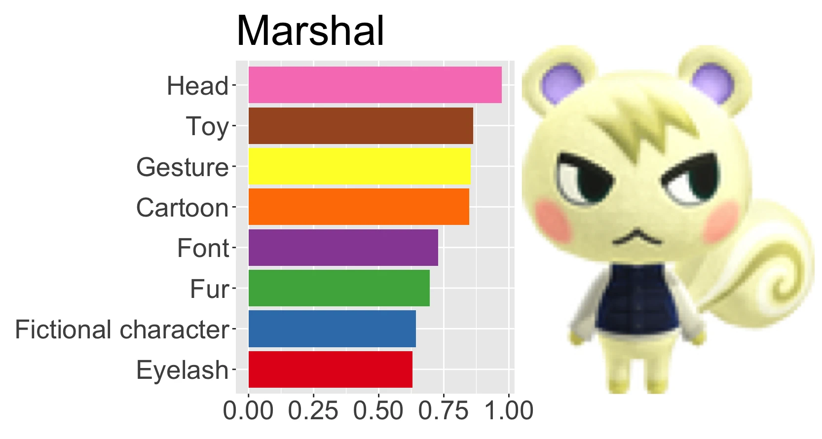
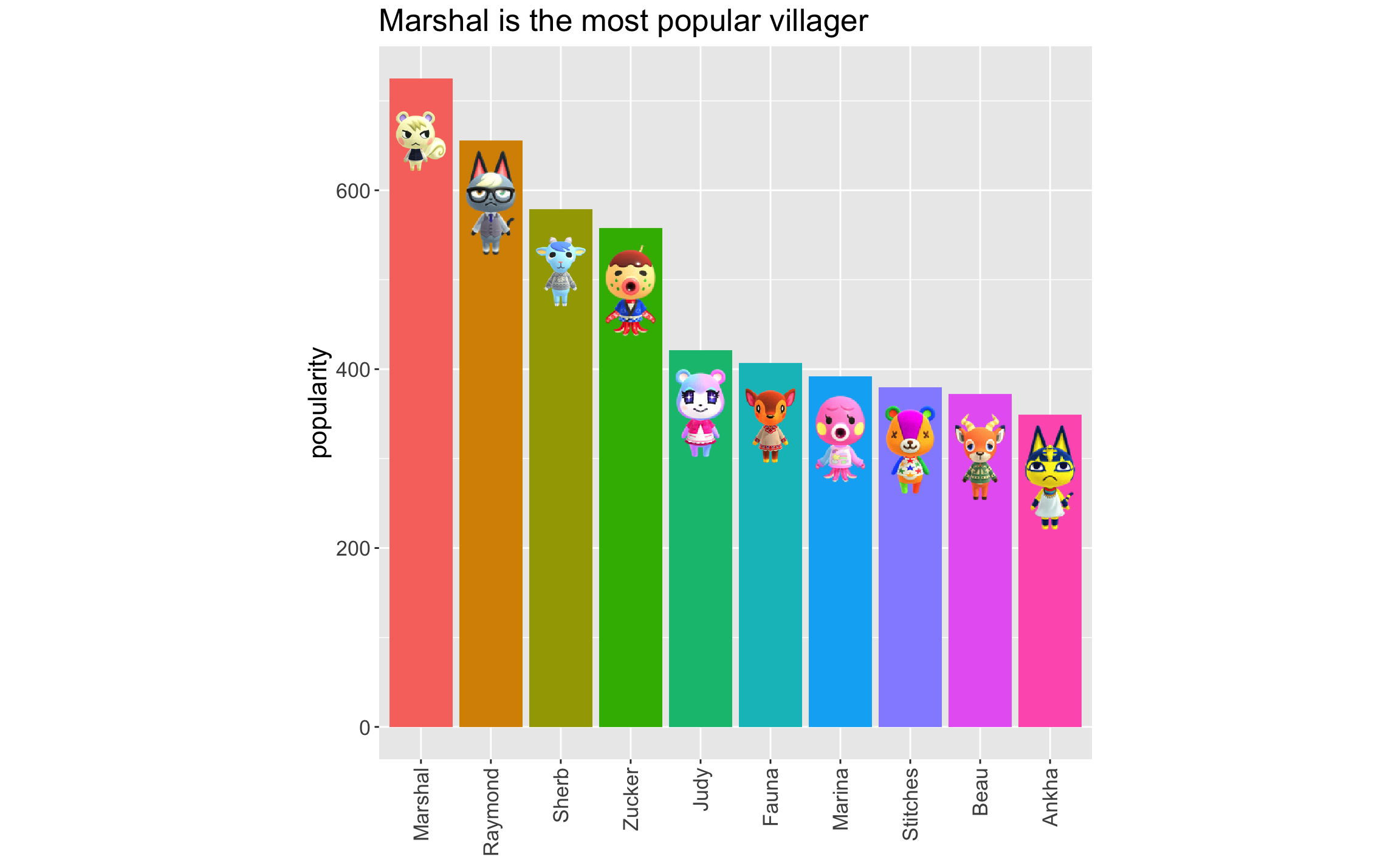
Those thumbnails add a bit of flair to any plot. It should come as no surprise to any Animal Crossing fan that Marshal is the favourite:
villagers %>%
  arrange(-popularity) %>%
  head(10) %>%
  mutate(name = factor(name, levels = name)) %>%
  ggplot(aes(x = name, y = popularity, fill = name)) +
  geom_bar(stat = "identity") +
  geom_image(
    aes(x = name, y = popularity - 70, image = url),
    size = 0.07
  ) +
  ggtitle("Marshal is the most popular villager") +
  theme(
    text = element_text(size = 16),
    legend.position = "none",
    axis.title.x = element_blank(),
    axis.text.x = element_text(angle = 90, vjust = 0.5, hjust = 1),
    aspect.ratio = 1
  )
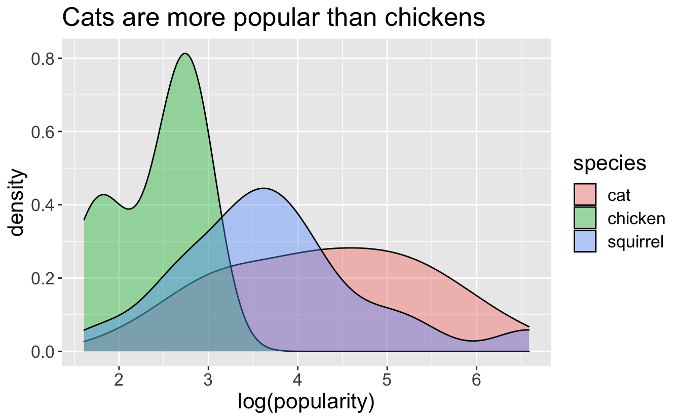
Animal Crossing villagers are sorted into 35 different species. Some are more loved than others. The popularity densities have long tails, so taking the log here makes them plot a lot better:
villagers %>%
    filter(species %in% c("cat", "chicken", "squirrel")) %>%
    ggplot(aes(x = log(popularity), group = species, fill = species)) +
    geom_density(alpha = 0.4) +
    theme(text = element_text(size = 16)) +
    ggtitle("Cats are more popular than chickens")
Octopuses are particularly loved, though. There are only 3 octopus villagers, but their mean popularity is 366, as opposed to the overall mean popularity of 57. People really like Zucker!
Authenticating with Google Cloud
By this point I’ve already set up an account and project with the Google Cloud Platform (GCP), and enabled the relevant APIs. I won’t go into that detail here, since the GCP documentation is pretty good. However, I still need to authenticate myself to the GCP before I can use any of its services.
There’s no all-encompassing R SDK for the Google Cloud Platform. A few services can be used with packages provided by the CloudyR project, but there’s nothing for the Vision API. I’m happy to use Google’s HTTP APIs directly, but the authentication usually trips me up. Fortunately, the gargle package is excellent, and makes the authentication much simpler than it would be to do it manually.
Following the instructions provided by Google, I created a service account with read/write access to Cloud Storage and permissions to use the Vision API. The actual credentials are kept in a JSON. Within my .Renviron file (hint: usethis::edit_r_environ() will open this in RStudio) I set the “GOOGLE_APPLICATION_CREDENTIALS” environment variable to the path of this JSON. Now, I can use the gargle package to create a token with the appropriate scopes:
gcp_token <- gargle::credentials_service_account(
  scopes = c(
    "https://www.googleapis.com/auth/cloud-vision",
    "https://www.googleapis.com/auth/devstorage.read_write"
  ),
  path = Sys.getenv("GOOGLE_APPLICATION_CREDENTIALS")
)
This token can be passed into httr verbs (in fact, it’s a httr::TokenServiceAccount) where it will be used for authentication. httr handles all of the stuff I don’t want to think about, like token refreshing and authentication headers.
Uploading the images
I can query the Vision API with image data directly, but another option is to keep the thumbnails in a Cloud Storage bucket. I created an animal-crossing bucket through the Google Cloud Platform console. I’ll create a function for uploading villager images. I assume villager to be a single row of the villagers data frame, so that I can effectively treat it like a list. This function will:
- download
villager$urlto a temp file and useon.exitto clean up afterwards, - define the name of the object I’m creating, using the villager’s id,
- use
httr::POSTto post the image using mygcp_token, and finally - check that the resulting status code is 200 (success)
upload_villager_image <- function(villager) {
  temp <- tempfile()
  on.exit(unlink(temp))
  download.file(villager$url, temp)
  object_name <- paste0(villager$id, ".png")

  response <- POST(
    glue("https://storage.googleapis.com/upload/storage/v1/b/animal-crossing/o?uploadType=media&name={object_name}"),
    body = upload_file(temp, type = "image/png"),
    config(token = gcp_token)
  )
  if (status_code(response) != 200) {
    stop(glue("Upload of {villager$id} failed with status code {status_code(response)}"))
  }
}
If I can upload a single villager image, I can upload them all. I use purrr to iterate through the rows of the villagers data frame, uploading each of the 391 villager images.
walk(
  1:nrow(villagers),
  function(row_index) {
    villager <- villagers[row_index,]
    upload_villager_image(villager)
  }
)
A quick aside: I don’t often see code that uses purrr to iterate through the rows of a data frame like this, which makes me think I’m doing something unconventional. A better option may be to pull out villager$name and villager$url, and pass those as arguments to a binary upload_villager_image function.
Annotating the villagers
With the images uploaded to Cloud Storage, I can query the Cloud Vision API with the path to a given thumbnail. For example, I can give gs://animal-crossing/tangy.png as an argument to the images:annotate endpoint.
The response is a list of labels, each consisting of a description (the label itself), a confidence score and a topicality score. I’ll flatten this to a one-row data frame (tibble) of confidence scores, with columns the labels. This will make it easier to later concatenate the labels with the villagers data frame.
Note also the potential for the API to return duplicate labels — in this case, I take the maximum score.
annotate <- function(villager_id) {
  json <- jsonlite::toJSON(
      list(
          requests = list(
              image = list(
                  source = list(
                      gcsImageUri = glue::glue("gs://animal-crossing/{villager_id}.png")
                  )
              ),
              features = list(list(
                  maxResults = 50,
                  type = "LABEL_DETECTION"
              ))
          )
      ),
      auto_unbox = TRUE
  )

  response <- POST(
      "https://vision.googleapis.com/v1/images:annotate",
      body = json,
      config(token = gcp_token),
      add_headers(`Content-Type` = "application/json; charset=utf-8")
  )

  if (status_code(response) != 200) {
      stop("Error labelling ", villager)
  }

  content(response)$responses[[1]]$labelAnnotations %>%
    map(as_tibble) %>%
    reduce(bind_rows) %>%
    select(description, score) %>%
    pivot_wider(names_from = description, values_from = score, values_fn = max) %>%
    janitor::clean_names()
}
I ask for 50 labels, but the API appears not return labels with a confidence score of less than 0.5, so I may get fewer:
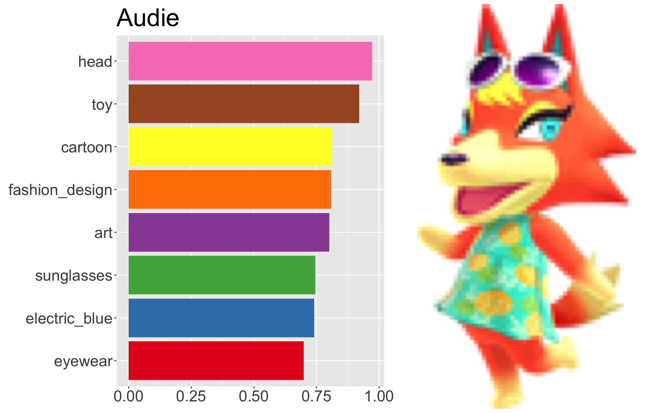
annotate("audie")
#> # A tibble: 1 x 19
#>    head   toy cartoon fashion_design   art sunglasses electric_blue eyewear
#>   <dbl> <dbl>   <dbl>          <dbl> <dbl>      <dbl>         <dbl>   <dbl>
#> 1 0.972 0.921   0.812          0.808 0.801      0.746         0.741   0.699
#> # … with 11 more variables: magenta <dbl>, fictional_character <dbl>,
#> #   goggles <dbl>, doll <dbl>, pattern <dbl>, entertainment <dbl>,
#> #   figurine <dbl>, visual_arts <dbl>, performing_arts <dbl>, child_art <dbl>,
#> #   painting <dbl>
This isn’t very pretty to look at, so I’ll make a nice plot:
plot_villager <- function(villager_id) {
  villager <- villagers %>% filter(id == villager_id)
  if (nrow(villager) == 0) {
    stop("Couldn't find villager with id ", villager_id)
  }

  villager_plot <- villager_id %>%
    annotate() %>%
    pivot_longer(everything(), names_to = "label", values_to = "score") %>%
    top_n(8, wt = score) %>%
    mutate(label = factor(label, levels = rev(.$label))) %>%
    ggplot(aes(x = label, y = score, fill = label)) +
    geom_bar(stat = "identity") +
    scale_fill_brewer(palette="Set1") +
    theme(
      legend.position = "none",
      axis.title.x = element_blank(),
      axis.title.y = element_blank(),
      axis.text = element_text(size = 20),
      plot.title = element_text(size = 32)
    ) +
    ggtitle(villager$name) +
    coord_flip()

  villager_image <- png::readPNG(
    curl::curl_fetch_memory(villager$url)$content,
    native = TRUE
  )

  villager_plot + villager_image
}plot_villager("audie")
An attempt at machine learning
Readers of my blog should expect this by now, but I tend not to care about model accuracy in these posts. My interest is always in the process of building a model, rather than the model itself. A warning ahead: the model I’m about to train here will perform terribly.
I don’t believe model tuning or trying different techniques would help here. The dataset is very sparse and wide, so there’s not a lot of information to model.
Label all villagers
I’ve defined a function for annotating a single villager, but I have 391 to label. Google Cloud does have a batch annotation API, but I decided to save the coding effort and just re-use my single-villager annotation function with purrr.
The following can take a few minutes. At times progress was stalling, and I suspect I was brushing up against some API limits. The Sys.sleep(0.5) is intended to address that, but I’m only speculating.
labels <- map(villagers$id, function(x) {Sys.sleep(0.5); list(annotate(x))}) %>%
  reduce(bind_rows) %>%
  rename_all(~glue("label_{.x}"))
I’ve prefixed every label with “label_” so that I can identify these columns later in data pre-processing. Setting up a sensible column naming convention will let me use the powerful tidyselect::starts_with selector.
labels is a wide data frame with 413 columns. But 94% entries are NA. This is because the Cloud Vision API returns only the labels it deems most relevant. It also seems to not return any labels with a “score” of less than 0.5. The end result of dplyr::bind_rows is a wide, sparse data frame of floats and NAs.
I’ll have to deal with this problem in pre-processing. For now I’ll combine labels with the villagers data frame:
Pre-processing
I’ll use the recipes package to pre-process the data before modelling. This is one of my favourite packages, and a real star of tidymodels. First I’ll do a simple train/test split, since my pre-processing strategy can’t depend on the test data:
split <- initial_split(villagers_labelled, prop = 0.8)
train <- training(split)
dim(train)
#> [1] 312 425
test <- testing(split)
dim(test)
#> [1]  79 425
To mitigate the impact of the sparsity, I’ll remove any labels that are blank more than half the time in the training data. I’ll make a note of these now:
too_many_missing <- train %>%
  select(starts_with("label")) %>%
  select_if(~sum(is.na(.x))/length(.x) > 0.5) %>%
  colnames()
I can’t find documentation to confirm this, but it appears as though the Google Cloud Vision API won’t return a label with a score of less than 0.5. One way to deal with the sparsity of these labels is to binarise them — TRUE if the label is present, otherwise FALSE. This turns the labels into features that effectively say, “Did the Cloud Vision API detect this label?”.
Species is also a difficult predictor here — in the training set there are 35 different species amongst 312 villagers. I’ll collapse the uncommon species into an “other” category.
The remaining pre-processing steps are fairly standard — discarding unneeded columns, converting strings to factors, and applying one-hot encoding. I’ll also keep using log(popularity) here, to deal with those long tails in the popularity scores.
pre_processing <- recipe(train, popularity ~ .) %>%
  step_rm(row_n, id, name, birthday, song, phrase, full_id, url) %>%
  step_rm(one_of(too_many_missing)) %>%
  step_mutate_at(starts_with("label"), fn = ~as.integer(!is.na(.x))) %>%
  step_string2factor(has_type("character")) %>%
  step_other(species, threshold = 0.03) %>%
  step_dummy(all_nominal_predictors(), one_hot = TRUE) %>%
  step_log(popularity, skip = TRUE)
An xgboost model
The processed train data has 37 columns, but is of (matrix) rank 34. Informally, this means that the training data is bigger than the information it contains. Linear models will throw warnings here. Tree-based methods will hide the problem, but there’s no escaping the fact that any model trained on this data will be terrible.
I’ll set up an xgboost model with the parsnip package, allowing for tuning the tree_depth and mtry parameters. Here, mtry refers to the number of predictors available to the model at each split. Finally, I’ll combine the pre-processing and the model into a workflow.
xgboost_model <- boost_tree(trees = 200, mtry = tune(), tree_depth = tune()) %>%
  set_engine("xgboost") %>%
  set_mode("regression")

xgboost_workflow <- workflow() %>%
  add_recipe(pre_processing) %>%
  add_model(xgboost_model)
xgboost_workflow
#> ══ Workflow ════════════════════════════════════════════════════════════════════
#> Preprocessor: Recipe
#> Model: boost_tree()
#>
#> ── Preprocessor ────────────────────────────────────────────────────────────────
#> 7 Recipe Steps
#>
#> • step_rm()
#> • step_rm()
#> • step_mutate_at()
#> • step_string2factor()
#> • step_other()
#> • step_dummy()
#> • step_log()
#>
#> ── Model ───────────────────────────────────────────────────────────────────────
#> Boosted Tree Model Specification (regression)
#>
#> Main Arguments:
#>   mtry = tune()
#>   trees = 200
#>   tree_depth = tune()
#>
#> Computational engine: xgboost
I’ll tune the model, relying on the default grid for tree_depth and mtry, and using 5-fold cross-validation:
folds <- vfold_cv(train, v = 5)
tune_results <- tune_grid(xgboost_workflow, resamples = folds)
#> i Creating pre-processing data to finalize unknown parameter: mtry
I’ll use whichever mtry and tree_depth parameters minimise root mean-squared error to finalise my workflow, and fit it to the train data.
fitted_xgboost_workflow <- xgboost_workflow %>%
  finalize_workflow(select_best(tune_results, metric = "rmse")) %>%
  fit(train)
It’s time to see just how bad this model is. Recall that I took the log of the popularity in the training data, so to truly evaluate the performance I have to take the exp of the predictions.
test_performance <- test %>%
  mutate(
    predicted =  predict(fitted_xgboost_workflow, test)$.pred %>% exp(),
    residual = popularity - predicted
  )
metric_set(rmse, mae)(test_performance, popularity, predicted)
#> # A tibble: 2 x 3
#>   .metric .estimator .estimate
#>   <chr>   <chr>          <dbl>
#> 1 rmse    standard       108.
#> 2 mae     standard        58.0
Oof, that model is pretty bad. I wonder if it’s because the distribution of popularity isn’t uniform? I’ll compare the predicted and actual values to see if there’s a difference at the extreme ends:
test_performance %>%
  ggplot(aes(x = predicted, y = popularity)) +
  geom_point() +
  geom_abline(intercept = 0, slope = 1)
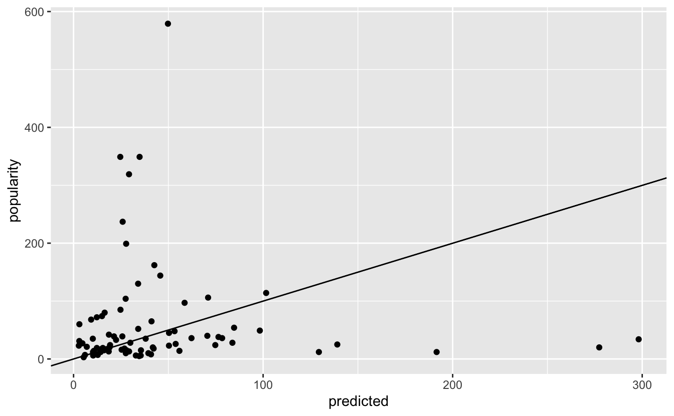
Sure enough, that seems to be the case. For values below about 50, the model seems to be not too bad, and certainly better than it performs for the more popular villagers.
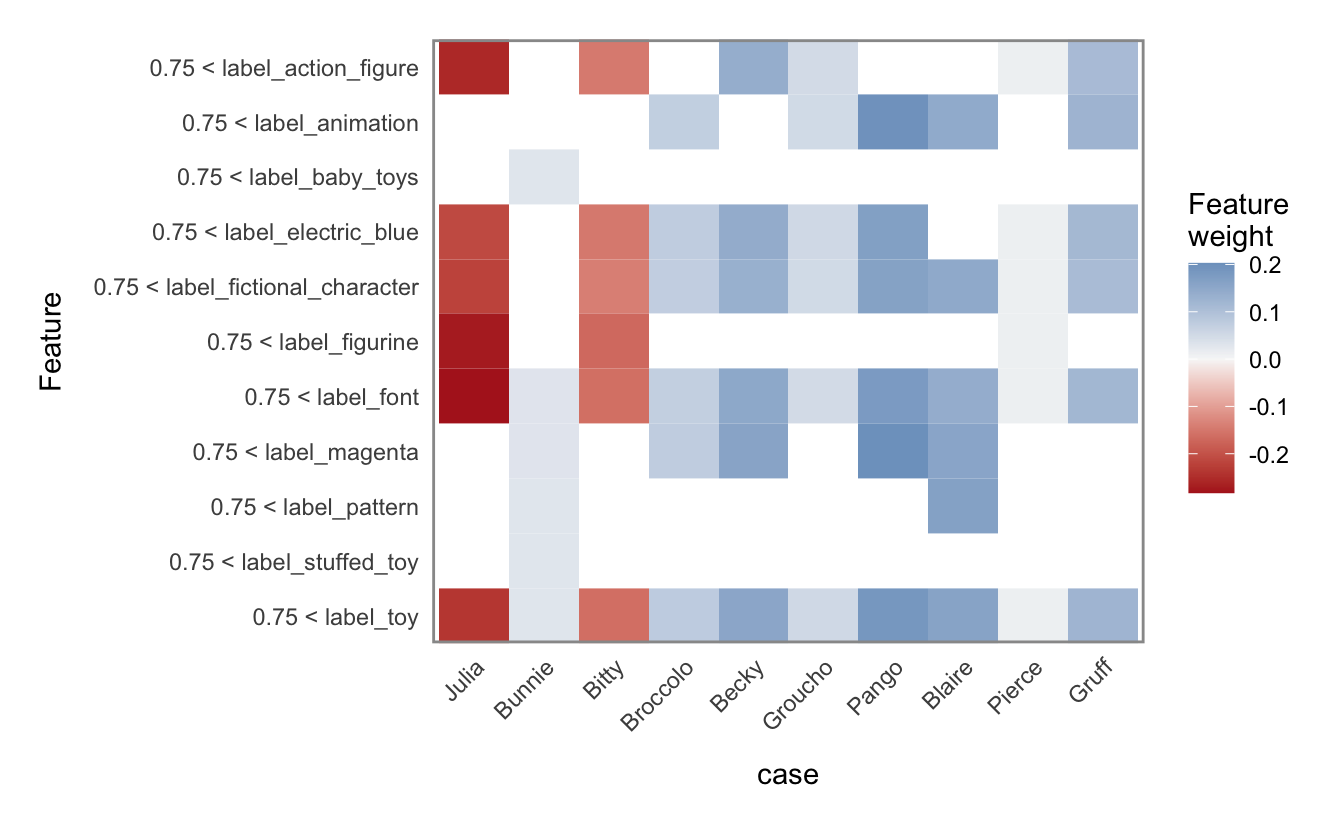
Model interpretability
I tried to use some model interpretability techniques to see what effect these labels were having on villager popularity. Unfortunately, I had trouble applying either LIME or SHAP:
- The
limepackage throws many, many warnings. I’m not surprised. The inputs are rank-deficient matrices and the LIME technique uses on linear models. - The
shaprpackage doesn’t support explanations for more than 30 features.
I’ll show the results of my lime analysis here, with the understanding that the results are almost certainly nonsense.
First I’ll separate the pre-processing function and model object from the workflow, since lime (nor shapr) can’t handle the in-built pre-processing of a workflow object:
pre_processing_function <- function(x) {
  pull_workflow_prepped_recipe(fitted_xgboost_workflow) %>%
    bake(x) %>%
    select(-popularity)
}

fitted_xgboost_model <- pull_workflow_fit(fitted_xgboost_workflow)
Then I fit the explainer. The quantile binning approach just doesn’t work with such sparse data, so I disable it.
explainer <- lime(
  pre_processing_function(train),
  fitted_xgboost_model,
  quantile_bins = FALSE
)
Now I’ll explain a few test cases and plot the results. I’ll suppress the warnings that would usually appear here.
test_case <- sample_n(test, 10)

explanations <- suppressWarnings(
  explain(
    pre_processing_function(test_case),
    explainer,
    n_features = 6
  )
)

plot_explanations(explanations) +
  scale_x_discrete(labels = test_case$name)
The Animal Crossing franchise and its fictional characters are the property of Nintendo. The thumbnail images of Animal Crossing villagers on this page are used for the purposes of study and commentary.
devtools::session_info()
#> ─ Session info ───────────────────────────────────────────────────────────────
#>  setting  value
#>  version  R version 4.1.0 (2021-05-18)
#>  os       macOS Big Sur 11.3
#>  system   aarch64, darwin20
#>  ui       X11
#>  language (EN)
#>  collate  en_AU.UTF-8
#>  ctype    en_AU.UTF-8
#>  tz       Australia/Melbourne
#>  date     2021-06-07
#>
#> ─ Packages ───────────────────────────────────────────────────────────────────
#>  package      * version    date       lib source
#>  askpass        1.1        2019-01-13 [1] CRAN (R 4.1.0)
#>  assertthat     0.2.1      2019-03-21 [1] CRAN (R 4.1.0)
#>  backports      1.2.1      2020-12-09 [1] CRAN (R 4.1.0)
#>  BiocManager    1.30.15    2021-05-11 [1] CRAN (R 4.1.0)
#>  broom        * 0.7.6      2021-04-05 [1] CRAN (R 4.1.0)
#>  cachem         1.0.4      2021-02-13 [1] CRAN (R 4.1.0)
#>  callr          3.7.0      2021-04-20 [1] CRAN (R 4.1.0)
#>  cellranger     1.1.0      2016-07-27 [1] CRAN (R 4.1.0)
#>  class          7.3-19     2021-05-03 [1] CRAN (R 4.1.0)
#>  cli            2.5.0      2021-04-26 [1] CRAN (R 4.1.0)
#>  codetools      0.2-18     2020-11-04 [1] CRAN (R 4.1.0)
#>  colorspace     2.0-1      2021-05-04 [1] CRAN (R 4.1.0)
#>  crayon         1.4.1      2021-02-08 [1] CRAN (R 4.1.0)
#>  curl           4.3.1      2021-04-30 [1] CRAN (R 4.1.0)
#>  data.table     1.14.0     2021-02-21 [1] CRAN (R 4.1.0)
#>  DBI            1.1.1      2021-01-15 [1] CRAN (R 4.1.0)
#>  dbplyr         2.1.1      2021-04-06 [1] CRAN (R 4.1.0)
#>  desc           1.3.0      2021-03-05 [1] CRAN (R 4.1.0)
#>  devtools       2.4.0      2021-04-07 [1] CRAN (R 4.1.0)
#>  dials        * 0.0.9      2020-09-16 [1] CRAN (R 4.1.0)
#>  DiceDesign     1.9        2021-02-13 [1] CRAN (R 4.1.0)
#>  digest         0.6.27     2020-10-24 [1] CRAN (R 4.1.0)
#>  downlit        0.2.1      2020-11-04 [1] CRAN (R 4.1.0)
#>  dplyr        * 1.0.5      2021-03-05 [1] CRAN (R 4.1.0)
#>  ellipsis       0.3.2      2021-04-29 [1] CRAN (R 4.1.0)
#>  evaluate       0.14       2019-05-28 [1] CRAN (R 4.1.0)
#>  fansi          0.4.2      2021-01-15 [1] CRAN (R 4.1.0)
#>  farver         2.1.0      2021-02-28 [1] CRAN (R 4.1.0)
#>  fastmap        1.1.0      2021-01-25 [1] CRAN (R 4.1.0)
#>  forcats      * 0.5.1      2021-01-27 [1] CRAN (R 4.1.0)
#>  foreach        1.5.1      2020-10-15 [1] CRAN (R 4.1.0)
#>  fs             1.5.0      2020-07-31 [1] CRAN (R 4.1.0)
#>  furrr          0.2.2      2021-01-29 [1] CRAN (R 4.1.0)
#>  future         1.21.0     2020-12-10 [1] CRAN (R 4.1.0)
#>  gargle         1.1.0      2021-04-02 [1] CRAN (R 4.1.0)
#>  generics       0.1.0      2020-10-31 [1] CRAN (R 4.1.0)
#>  ggimage      * 0.2.8      2020-04-02 [1] CRAN (R 4.1.0)
#>  ggplot2      * 3.3.3      2020-12-30 [1] CRAN (R 4.1.0)
#>  ggplotify      0.0.7      2021-05-11 [1] CRAN (R 4.1.0)
#>  glmnet         4.1-1      2021-02-21 [1] CRAN (R 4.1.0)
#>  globals        0.14.0     2020-11-22 [1] CRAN (R 4.1.0)
#>  glue         * 1.4.2      2020-08-27 [1] CRAN (R 4.1.0)
#>  gower          0.2.2      2020-06-23 [1] CRAN (R 4.1.0)
#>  GPfit          1.0-8      2019-02-08 [1] CRAN (R 4.1.0)
#>  gridGraphics   0.5-1      2020-12-13 [1] CRAN (R 4.1.0)
#>  gtable         0.3.0      2019-03-25 [1] CRAN (R 4.1.0)
#>  hardhat        0.1.5      2020-11-09 [1] CRAN (R 4.1.0)
#>  haven          2.4.1      2021-04-23 [1] CRAN (R 4.1.0)
#>  highr          0.9        2021-04-16 [1] CRAN (R 4.1.0)
#>  hms            1.0.0      2021-01-13 [1] CRAN (R 4.1.0)
#>  htmltools      0.5.1.1    2021-01-22 [1] CRAN (R 4.1.0)
#>  httr         * 1.4.2      2020-07-20 [1] CRAN (R 4.1.0)
#>  hugodown       0.0.0.9000 2021-05-16 [1] Github (r-lib/hugodown@97ea0cd)
#>  infer        * 0.5.4      2021-01-13 [1] CRAN (R 4.1.0)
#>  ipred          0.9-11     2021-03-12 [1] CRAN (R 4.1.0)
#>  iterators      1.0.13     2020-10-15 [1] CRAN (R 4.1.0)
#>  jsonlite       1.7.2      2020-12-09 [1] CRAN (R 4.1.0)
#>  knitr          1.33       2021-04-24 [1] CRAN (R 4.1.0)
#>  labeling       0.4.2      2020-10-20 [1] CRAN (R 4.1.0)
#>  lattice        0.20-44    2021-05-02 [1] CRAN (R 4.1.0)
#>  lava           1.6.9      2021-03-11 [1] CRAN (R 4.1.0)
#>  lhs            1.1.1      2020-10-05 [1] CRAN (R 4.1.0)
#>  lifecycle      1.0.0      2021-02-15 [1] CRAN (R 4.1.0)
#>  lime         * 0.5.2      2021-02-24 [1] CRAN (R 4.1.0)
#>  listenv        0.8.0      2019-12-05 [1] CRAN (R 4.1.0)
#>  lubridate      1.7.10     2021-02-26 [1] CRAN (R 4.1.0)
#>  magick         2.7.2      2021-05-02 [1] CRAN (R 4.1.0)
#>  magrittr       2.0.1      2020-11-17 [1] CRAN (R 4.1.0)
#>  MASS           7.3-54     2021-05-03 [1] CRAN (R 4.1.0)
#>  Matrix         1.3-3      2021-05-04 [1] CRAN (R 4.1.0)
#>  memoise        2.0.0      2021-01-26 [1] CRAN (R 4.1.0)
#>  modeldata    * 0.1.0      2020-10-22 [1] CRAN (R 4.1.0)
#>  modelr         0.1.8      2020-05-19 [1] CRAN (R 4.1.0)
#>  munsell        0.5.0      2018-06-12 [1] CRAN (R 4.1.0)
#>  nnet           7.3-16     2021-05-03 [1] CRAN (R 4.1.0)
#>  openssl        1.4.4      2021-04-30 [1] CRAN (R 4.1.0)
#>  parallelly     1.25.0     2021-04-30 [1] CRAN (R 4.1.0)
#>  parsnip      * 0.1.6      2021-05-27 [1] CRAN (R 4.1.0)
#>  patchwork    * 1.1.1      2020-12-17 [1] CRAN (R 4.1.0)
#>  pillar         1.6.1      2021-05-16 [1] CRAN (R 4.1.0)
#>  pkgbuild       1.2.0      2020-12-15 [1] CRAN (R 4.1.0)
#>  pkgconfig      2.0.3      2019-09-22 [1] CRAN (R 4.1.0)
#>  pkgload        1.2.1      2021-04-06 [1] CRAN (R 4.1.0)
#>  plyr           1.8.6      2020-03-03 [1] CRAN (R 4.1.0)
#>  prettyunits    1.1.1      2020-01-24 [1] CRAN (R 4.1.0)
#>  pROC           1.17.0.1   2021-01-13 [1] CRAN (R 4.1.0)
#>  processx       3.5.2      2021-04-30 [1] CRAN (R 4.1.0)
#>  prodlim        2019.11.13 2019-11-17 [1] CRAN (R 4.1.0)
#>  ps             1.6.0      2021-02-28 [1] CRAN (R 4.1.0)
#>  purrr        * 0.3.4      2020-04-17 [1] CRAN (R 4.1.0)
#>  R6             2.5.0      2020-10-28 [1] CRAN (R 4.1.0)
#>  Rcpp           1.0.6      2021-01-15 [1] CRAN (R 4.1.0)
#>  readr        * 1.4.0      2020-10-05 [1] CRAN (R 4.1.0)
#>  readxl         1.3.1      2019-03-13 [1] CRAN (R 4.1.0)
#>  recipes      * 0.1.16     2021-04-16 [1] CRAN (R 4.1.0)
#>  remotes        2.3.0      2021-04-01 [1] CRAN (R 4.1.0)
#>  reprex         2.0.0      2021-04-02 [1] CRAN (R 4.1.0)
#>  rlang          0.4.11     2021-04-30 [1] CRAN (R 4.1.0)
#>  rmarkdown      2.8        2021-05-07 [1] CRAN (R 4.1.0)
#>  rpart          4.1-15     2019-04-12 [1] CRAN (R 4.1.0)
#>  rprojroot      2.0.2      2020-11-15 [1] CRAN (R 4.1.0)
#>  rsample      * 0.1.0      2021-05-08 [1] CRAN (R 4.1.0)
#>  rstudioapi     0.13       2020-11-12 [1] CRAN (R 4.1.0)
#>  rvcheck        0.1.8      2020-03-01 [1] CRAN (R 4.1.0)
#>  rvest          1.0.0      2021-03-09 [1] CRAN (R 4.1.0)
#>  scales       * 1.1.1      2020-05-11 [1] CRAN (R 4.1.0)
#>  sessioninfo    1.1.1      2018-11-05 [1] CRAN (R 4.1.0)
#>  shape          1.4.6      2021-05-19 [1] CRAN (R 4.1.0)
#>  stringi        1.6.1      2021-05-10 [1] CRAN (R 4.1.0)
#>  stringr      * 1.4.0      2019-02-10 [1] CRAN (R 4.1.0)
#>  survival       3.2-11     2021-04-26 [1] CRAN (R 4.1.0)
#>  testthat       3.0.2      2021-02-14 [1] CRAN (R 4.1.0)
#>  tibble       * 3.1.2      2021-05-16 [1] CRAN (R 4.1.0)
#>  tidymodels   * 0.1.3      2021-04-19 [1] CRAN (R 4.1.0)
#>  tidyr        * 1.1.3      2021-03-03 [1] CRAN (R 4.1.0)
#>  tidyselect     1.1.1      2021-04-30 [1] CRAN (R 4.1.0)
#>  tidyverse    * 1.3.1      2021-04-15 [1] CRAN (R 4.1.0)
#>  timeDate       3043.102   2018-02-21 [1] CRAN (R 4.1.0)
#>  tune         * 0.1.5      2021-04-23 [1] CRAN (R 4.1.0)
#>  usethis        2.0.1      2021-02-10 [1] CRAN (R 4.1.0)
#>  utf8           1.2.1      2021-03-12 [1] CRAN (R 4.1.0)
#>  vctrs          0.3.8      2021-04-29 [1] CRAN (R 4.1.0)
#>  withr          2.4.2      2021-04-18 [1] CRAN (R 4.1.0)
#>  workflows    * 0.2.2      2021-03-10 [1] CRAN (R 4.1.0)
#>  workflowsets * 0.0.2      2021-04-16 [1] CRAN (R 4.1.0)
#>  xfun           0.22       2021-03-11 [1] CRAN (R 4.1.0)
#>  xgboost        1.4.1.1    2021-04-22 [1] CRAN (R 4.1.0)
#>  xml2           1.3.2      2020-04-23 [1] CRAN (R 4.1.0)
#>  yaml           2.2.1      2020-02-01 [1] CRAN (R 4.1.0)
#>  yardstick    * 0.0.8      2021-03-28 [1] CRAN (R 4.1.0)
#>
#> [1] /Library/Frameworks/R.framework/Versions/4.1-arm64/Resources/library