I have a simple machine learning workflow that I recreate whenever I’m testing something new. I take some interesting data and a target, throw in some pre-processing, tune hyperparameters with cross-validation, and train a random forest. It’s all the basic ingredients for a machine learning model. Since I like Julia so much, I’ll recreate my simple machine learning workflow with Julia’s MLJ package.
MLJ is like R’s parsnip, in that it unifies many machine learning packages with disparate APIs under a single syntactic umbrella. And, like Python’s sklearn, it also supports pre-processing pipelines and hyperparameter optimisation.
Creating a Julia project
I always give some thought to project workflow, so this was a good opportunity to explore the Julia way of setting up a project.
Just as in R, there’s a strong tendency with Julia to create every project as a package. Julia’s inbuilt package manager Pkg (a package itself) makes it easy to set up and activate a new package environment:
Pkg.generate("MyJuliaProject")
Pkg.activate("MyJuliaProject")
cd("MyJuliaProject") # change working directory
Julia uses environments, similar to Python’s virtual environments, to keep track of dependencies and their versions. An environment has its own versioned packages, so that I don’t need to worry if I need version 0.20 of DataFrames for one project and 0.10 for another project. If I try to load a package Julia will first look for the package in the “MyJuliaProject” environment, and if it’s not available there then Julia will look into my base environment (“v1.5” for my installed version of Julia). Activating a package/project activates its environment, and I find that combining these two concepts into one is a good simplification. I can add packages to my project’s environment:
Pkg.add(["DataFrames", "DataFramesMeta", "CSV", "Chain", "MLJ", "DecisionTree",
         "MLJDecisionTreeInterface", "Lathe", "Gadfly"])
Or I can use Pkg.resolve() to try to get things into alignment. I find that Julia is pretty good at catching if my project uses packages I haven’t added.
Unlike Python, Julia’s environments are built into the language. It’s possible that this is why I find Julia’s environments so easy I to use while I struggle with Python’s virtual environments. I don’t have to mess around with my PATH variable or worry about running a command before I start Julia, since everything is done within Julia’s inbuilt Pkg, which is itself a Julia package.
My work above created a “MyJuliaProject” directory with two important metadata files:
- Project.toml is similar to R’s
DESCRIPTIONfiles, in that it tracks package metadata (author, name, etc.) and high-level dependencies. - Manifest.toml is similar to R’s
renv.lockor Python’srequirements.txt, in that it tracks detailed dependency information. Just as with the analogues in other languages, this file should never be touched by a human being.
Together these two metadata files can recreate the project/package environment. Julia handles all the complexities about where the environments are stored on the disk, and makes sure that if two environments share a dependency then it isn’t installed twice.
At this point I could lean into the package structure and start creating functions in a src/ subdirectory and unit tests in the tests/ subdirectory, but I don’t believe that I’m writing enough code to justify that overhead. Instead I’ll stick to a single script. In any case, if I ever return to this project on any system I can activate it and recover all of the dependencies I’m using today.
A little bit of EDA
My data set consists of 800 Pokémon. Pokémon can have one or two types which categorise what kind of Pokémon they are, according to their abilities or natural environments. For example, Charmander is a pure fire type Pokémon, whereas Charmander’s final evolution Charizard is Fire/Flying. Pokémon also have attributes known as “stats” which quantify their traits, and these are loosely related to their types. For example, rock Pokémon tend to have high defence, whereas fighting Pokémon tend to have high attack.
A natural candidate for a model, then, is whether or not we can predict a Pokémon’s first type from its stats. Let’s start by loading the data, along with the Julia packages we’ll need along the way:
using DataFrames
using DataFramesMeta
using Chain
using CSV
using MLJ
using Lathe.preprocess: TrainTestSplit
using Gadfly

# Roughly equivalent to ggplot themes
Gadfly.push_theme(
    style(
        background_color = colorant"white",
        line_width = 1mm,
        minor_label_font_size = 14pt,
        major_label_font_size = 16pt,
        key_title_font_size = 14pt,
        key_label_font_size = 12pt
    )
)
pokemon = CSV.read("data/pokemon.csv", DataFrame)
#> 800×13 DataFrame. Omitted printing of 7 columns
#> │ Row │ # │ Name │ Type 1 │ Type 2 │ Total │ HP │
#> │ │ Int64 │ String │ String │ String? │ Int64 │ Int64 │
#> ├─────┼───────┼───────────────────────┼─────────┼─────────┼───────┼───────┤
#> │ 1 │ 1 │ Bulbasaur │ Grass │ Poison │ 318 │ 45 │
#> │ 2 │ 2 │ Ivysaur │ Grass │ Poison │ 405 │ 60 │
#> │ 3 │ 3 │ Venusaur │ Grass │ Poison │ 525 │ 80 │
#> │ 4 │ 3 │ VenusaurMega Venusaur │ Grass │ Poison │ 625 │ 80 │
#> │ 5 │ 4 │ Charmander │ Fire │ missing │ 309 │ 39 │
#> │ 6 │ 5 │ Charmeleon │ Fire │ missing │ 405 │ 58 │
#> │ 7 │ 6 │ Charizard │ Fire │ Flying │ 534 │ 78 │
#> ⋮
#> │ 793 │ 716 │ Xerneas │ Fairy │ missing │ 680 │ 126 │
#> │ 794 │ 717 │ Yveltal │ Dark │ Flying │ 680 │ 126 │
#> │ 795 │ 718 │ Zygarde50% Forme │ Dragon │ Ground │ 600 │ 108 │
#> │ 796 │ 719 │ Diancie │ Rock │ Fairy │ 600 │ 50 │
#> │ 797 │ 719 │ DiancieMega Diancie │ Rock │ Fairy │ 700 │ 50 │
#> │ 798 │ 720 │ HoopaHoopa Confined │ Psychic │ Ghost │ 600 │ 80 │
#> │ 799 │ 720 │ HoopaHoopa Unbound │ Psychic │ Dark │ 680 │ 80 │
#> │ 800 │ 721 │ Volcanion │ Fire │ Water │ 600 │ 80 │One thing I really like about the way this DataFrame displays is that, since Type 2 is allowed to be missing, the data type for the column has a question mark after String. This indicates that it’s actually of type Union{Missing, String}, since missing has its own data type in Julia. It’s a nice touch.
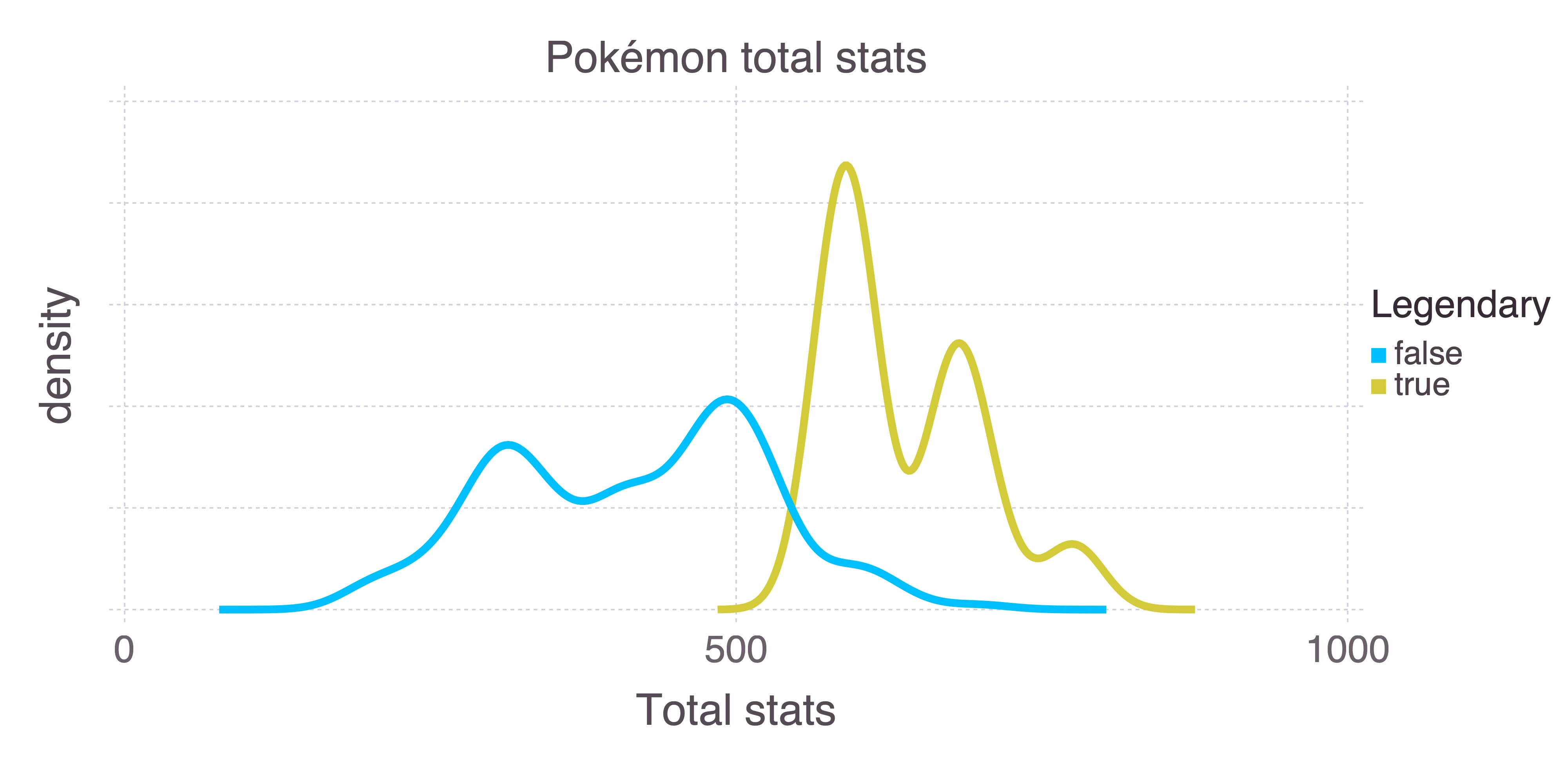
Certain Pokémon are legendary. They’re unique, and can usually only be encountered through some specific plot line or event. They also tend to be much more powerful than other Pokémon. We can use the sum of a Pokémon’s stats as a measure of how powerful it is:
plot(
    pokemon,
    x = "Total",
    color = "Legendary",
    Geom.density,
    Guide.yticks(label = false),
    Guide.xlabel("density"),
    Guide.xlabel("Total stats")
)
Pokémon stats are HP (health), attack, defence, special attack, special defence, and speed. There’s a distinction here between special and non-special attack and defence, where “special” is roughly defined as “supernatural”. For example, a kick is an attack, whereas a breath of fire is special. Comparing the attack attributes for fire and fighting Pokémon makes the distinction clear:
@chain pokemon begin
    @where in(["Fire", "Fighting"]).(:"Type 1")
    plot(
        x = "Attack",
        y = "Sp. Atk",
        color = "Type 1",
        Geom.point,
        Scale.color_discrete_manual("red", "silver")
    )
end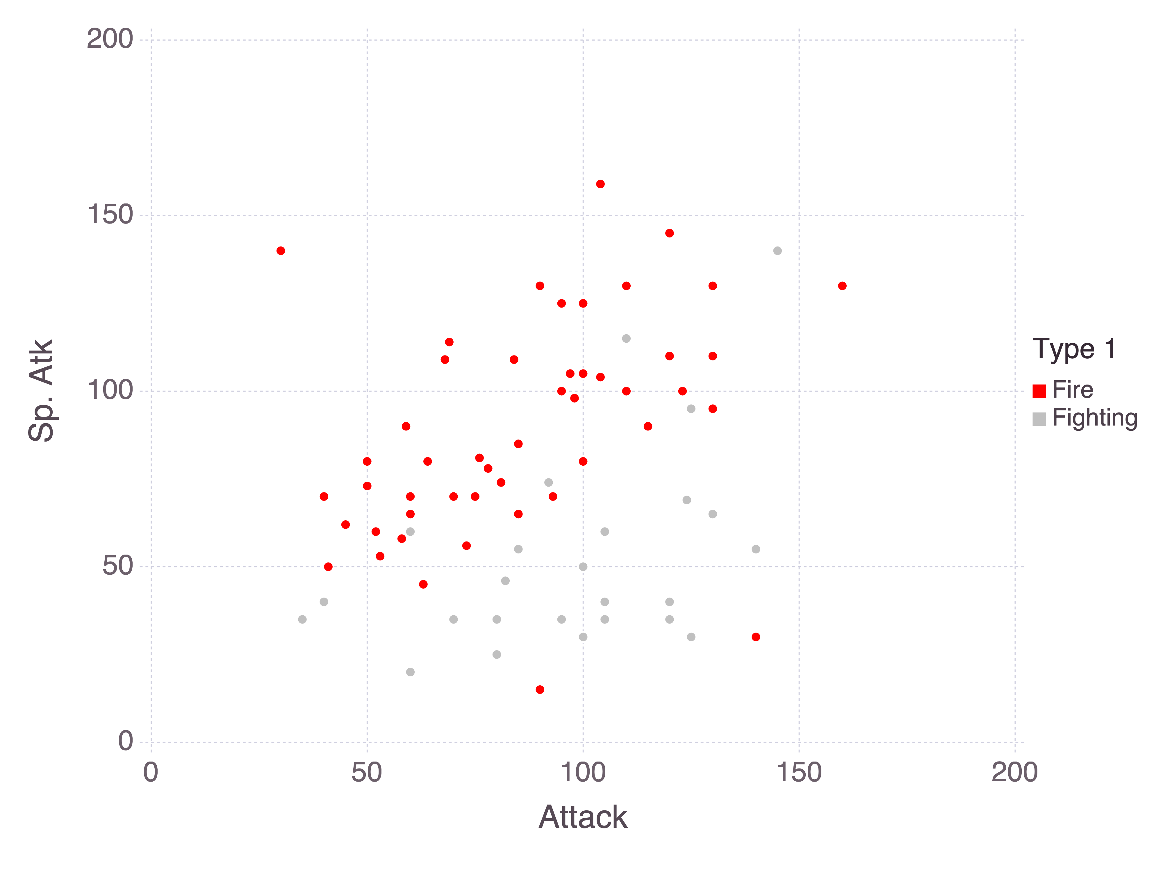
It’s not always so easy to separate types. Both fire and psychic Pokémon rely heavily on special attacks, and so we would expect their special attack stats to be similar.
Manipulating data in Julia
I want to be sure that the Total stat is genuinely the sum of all stats. I could instead choose to calculate the value myself rather than relying on the provided value, but I find that it’s rarely a good idea to silently correct data. This is just a toy example, but in general if something is wrong with my data then I want to know about it. Besides, it’s a good introduction to how data manipulation works in Julia.
Julia supports piping natively with |>, which is improved through the Pipe package, but an emerging alternative is Chain. With Chain every operation is placed on a new line, and the result of each line is piped through to the next:
@chain pokemon begin
    @with(:Total .== :HP .+ :Attack .+ :Defense .+ :"Sp. Atk" .+ :"Sp. Def" .+ :Speed)
    all
    @assert
end
The first line acts similarly to the with base function in R, in that it temporarily changes the environment such that I can refer to columns without referring to the pokemon data frame each time. The @ signals that this is a macro, which means that I’m using metaprogramming, ie. manipulating the input before evaluating it. The : character is used here to specify that these are symbols, here referring to column names. Overall I’m creating a vector of Boolean values, telling me for each Pokémon whether the Total stat is correct.
What stands out here for R and Python users is the dot before each operator1, such as .== and .+. This is a concept known as loop fusion. Recall that with Julia, I don’t need to avoid for loops like I would with numpy or R, where vectorised functions implemented in C/C++ are generally preferred. The . modifier here tells Julia to evaluate this operation in a for loop and, moreover, to evaluate all of the operations together. This works because every row is independent, so it makes sense to sum all of the stats for a single Pokémon in one iteration of the for loop.
As a mental model, I can vectorise any operation or user-defined function in Julia with loop fusion. Sure, in other languages I can vectorise any function with Vectorize (R) or numpy.vectorize (Python), but there are performance considerations — Vectorize is a wrapper for mapply, and numpy.vectorize effectively implements a for loop. Julia’s for loops are (subject to conditions) performant, whereas the standard advice for R and numpy is to not iterate.
There’s a learning curve here in terms of getting used to loop fusion. But the alternative is keeping a mental record of which functions are vectorised and which ones aren’t. Or writing your own vectorised functions in C/C++. Or relying on package authors to have written performant vectorised operations. Or just taking the performance hit of iterating in R or Python. I’d much rather take the loop fusion learning curve!
The final steps of this chain are an all function, which collapses an array of Booleans to a singleton, and an @assert which confirms that the output of the all function is true.
A straightforward random forest
I’ll start by training a random forest with (mostly) default values. MLJ follows the Python tradition of separating out an X data frame of training data and a y target column. I don’t think there’s anything wrong with this approach, but I feel like I’ve been spoilt by R’s use of formulae. It’s nice to keep all of the data together and not have to track multiple variables per data set. It also makes sense to me that pulling out a column and treating it as a “target variable” is a property of the model, not the data. But I’m nitpicking here — MLJ is excellent, and I shouldn’t fault it for not having an R convenience that I’m used to.
I’ll keep my X data set to just the stat columns and the :Total:
X = @select(pokemon, :Total, :HP, :Attack, :Defense, :"Sp. Atk", :"Sp. Def", :Speed)
y = pokemon[!, "Type 1"]
I couldn’t find a function like dplyr::pull in the DataFrames or DataFramesMeta packages. This function would be used to extract a column of a data frame as an array, rather than as a column. I instead use the [!, "Type 1"] syntax to pull the target values.
Recall that MLJ is a unified interface for disparate machine learning packages in Julia. I first need to @load a RandomForestClassifier from the DecisionTree package. From there I can define a classifier with 1000 trees.
rf_classifier = @load(RandomForestClassifier, pkg = "DecisionTree")
rf = rf_classifier(n_trees = 1000)
#> RandomForestClassifier(
#>     max_depth = -1,
#>     min_samples_leaf = 1,
#>     min_samples_split = 2,
#>     min_purity_increase = 0.0,
#>     n_subfeatures = -1,
#>     n_trees = 1000,
#>     sampling_fraction = 0.7,
#>     pdf_smoothing = 0.0) @140
I could move onto a fit/predict workflow here, but instead I’ll just evaluate the model to get an idea of its performance. By default, evaluate will use 6-fold cross-validation to evaluate the model, but I could control this by manually specifying folds, asking for an evaluation on a hold-out set instead, or even providing my own resampling strategy.
Note as well that I’m passing categorical(y), roughly equivalent to R’s as.factor(y). I can choose the measures under which the model is evaluated — in my case, I’m asking for simple classification accuracy. Normally the model would output an array of probabilities (one for each Pokémon type) but with the predict_mode operation I’m instead using the most probable type for my measure. There are other measures for evaluating accuracy, but nothing so easily interpretable as simple accuracy.
evaluate(rf, X, categorical(y), operation = predict_mode, measure = accuracy)
#> Evaluating over 6 folds: 100%[=========================] Time: 0:00:18
#> ┌───────────────┬───────────────┬────────────────────────────────────────────┐
#> │ _.measure     │ _.measurement │ _.per_fold                                 │
#> ├───────────────┼───────────────┼────────────────────────────────────────────┤
#> │ Accuracy @412 │ 0.216         │ [0.291, 0.201, 0.233, 0.241, 0.195, 0.135] │
#> └───────────────┴───────────────┴────────────────────────────────────────────┘
#> _.per_observation = [missing]
#> _.fitted_params_per_fold = [ … ]
#> _.report_per_fold = [ … ]</code></pre>
Given that there are 18 Pokémon types, 21.6% classification accuracy is pretty good. But let’s see if we can improve that.
Pre-processing in MLJ
MLJ developers have clearly given a lot of thought to model composition. Similar to sklearn, pipelines can be used to link together transformers and models.
I’m going to implement a very simple pipeline with a single stateless transformer. For stateful transformers, that is, transformers with fit and transform functions, the source code for the inbuilt OneHotEncoder looks to be a good template. In general I’m only scratching the surface of MLJ’s capacity to compose models.
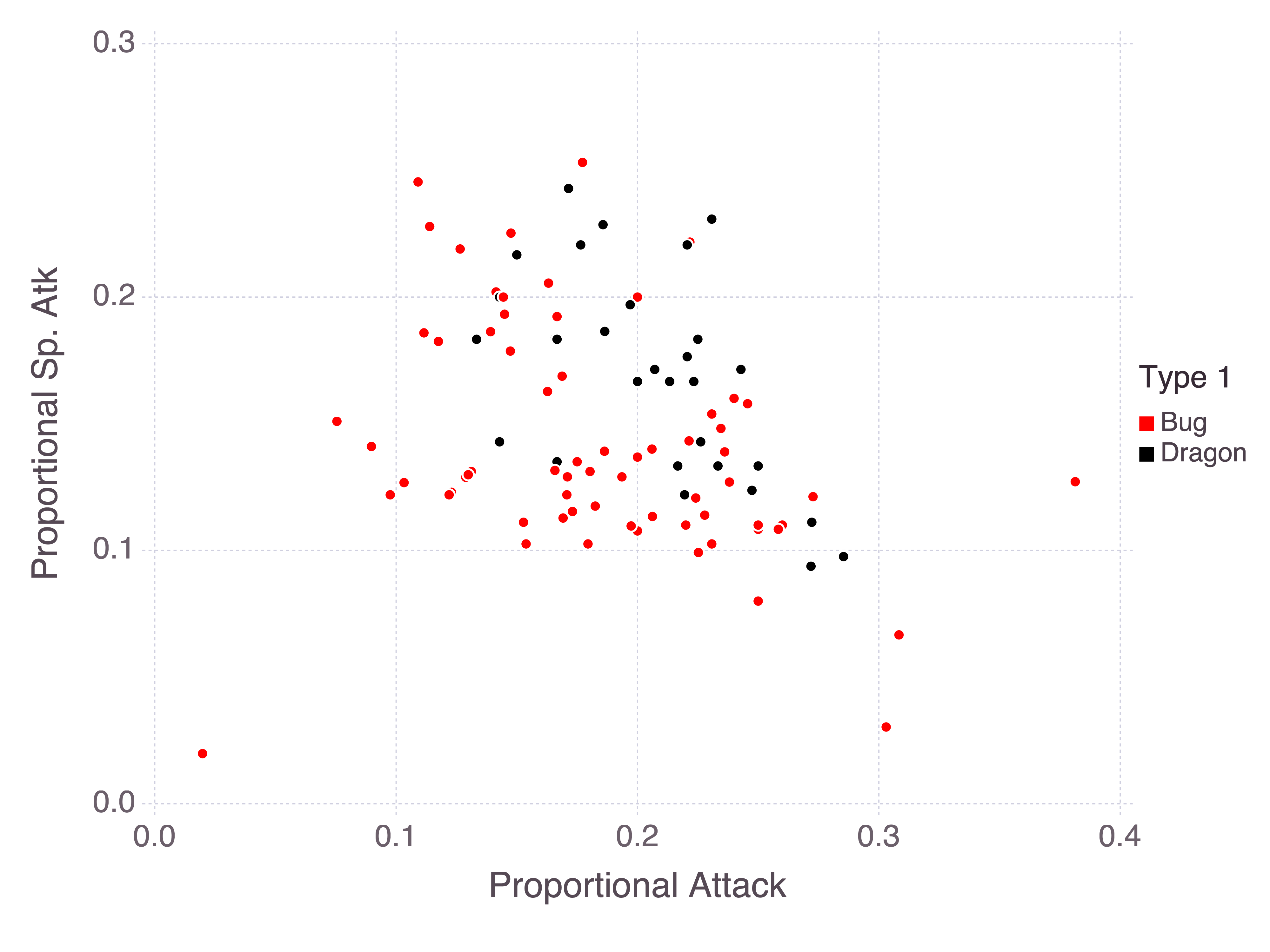
In my random forest I included all stats along with the Total as predictors, but it would make more sense to view each stat as a proportion of the Total. This way the model can infer how much weight is given to each stat. Consider, for example, bug and dragon Pokémon with their attack and special attack stats:
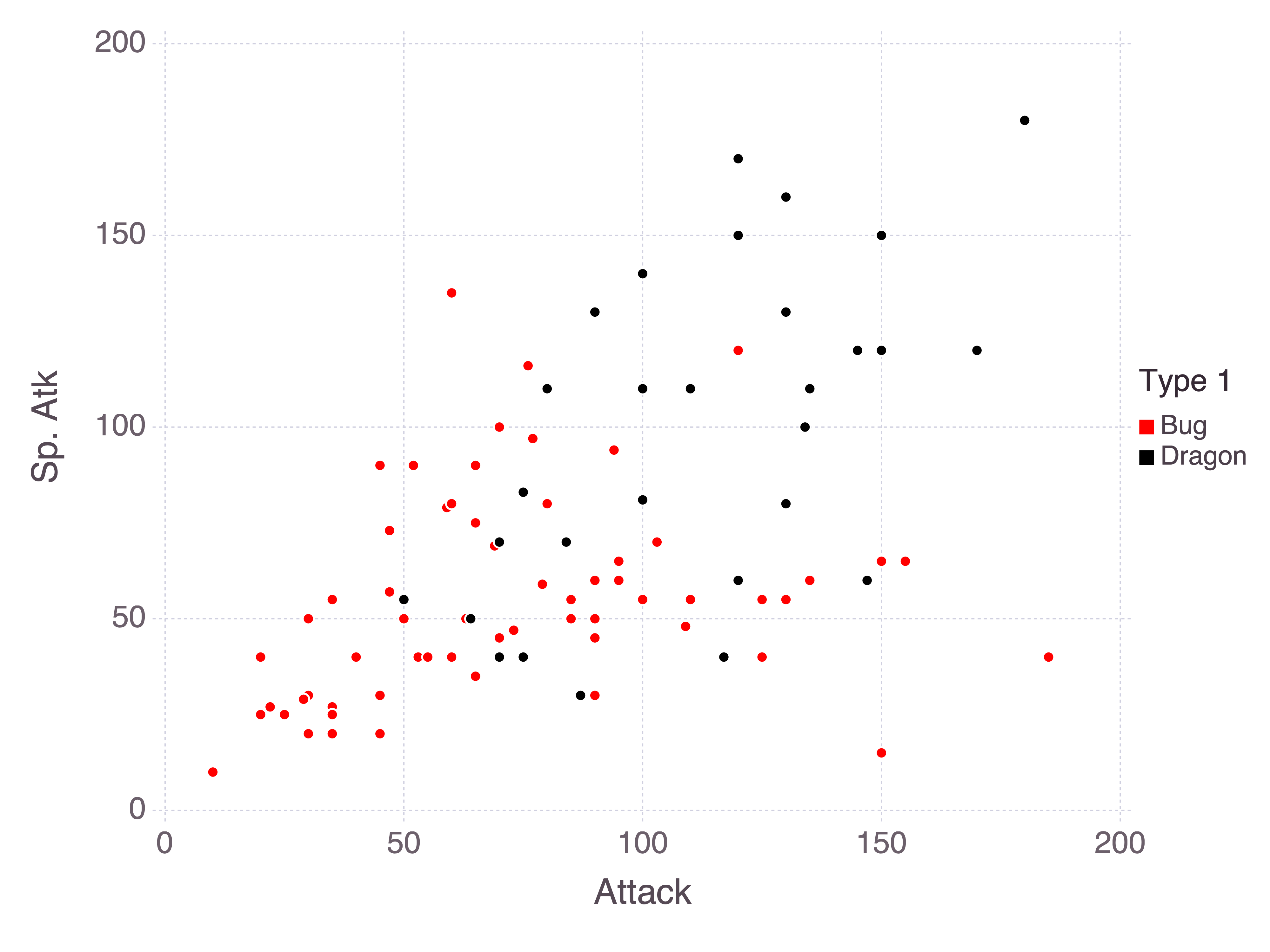
As a rule of thumb, bug Pokémon tend to be weaker while dragon Pokémon tend to be stronger. So we could consider instead these stats as proportions of the sum of stats:
I don’t know if this will help tease apart these classes, but it’s worth a try. This (pure) function takes in a data frame and scales the stats. Notice that I need to use the special cols function to include spaces in column names. The R equivalent would be to wrap the column names in backticks, but there doesn’t appear to be a general Julia solution. cols appears to be specific to the DataFramesMeta package.
function scale_stats(df::DataFrame)
    @select(df,
        HP = :HP ./ :Total,
        Attack = :Attack ./ :Total,
        Defencese = :Defense ./ :Total,
        cols("Sp. Atk") = :"Sp. Atk" ./ :Total,
        cols("Sp. Def") = :"Sp. Def" ./ :Total,
        Speed = :Speed ./ :Total,
        Total = :Total
    )
end
I define a pipeline with the @pipeline macro and give it a nice name:
pipe = @pipeline(
    scale_stats,
    rf_classifier(n_trees = 1000),
    name = "random_forest_with_proportional_stats"
)
#> random_forest_with_proportional_stats(
#>     random_forest_classifier = RandomForestClassifier(
#>             max_depth = -1,
#>             min_samples_leaf = 1,
#>             min_samples_split = 2,
#>             min_purity_increase = 0.0,
#>             n_subfeatures = -1,
#>             n_trees = 1000,
#>             sampling_fraction = 0.7,
#>             pdf_smoothing = 0.0)) @548
Self-tuning pipes
I might also eke out a little more performance by tuning my random forest. Two good candidate hyperparameters to tune in a random forest are max_depth (how deep the individual trees are allowed to grow) and n_subfeatures (how many randomly selected features are allowed as candidates for each split).
MLJ asks that I define a range for each hyperparameter I wish to tune. The input for each range is the pipeline that I’m intending to tune, along with the variable — note that I’m choosing the max_depth parameter within the random_forest_classifier within the pipe. Finally I specify the values. I explicitly provide the values I wish to test, but there are alternative methods.
max_depth_range = range(
    pipe,
    :(random_forest_classifier.max_depth),
    values = [-1, 10, 20]
)
n_subfeatures_range = range(
    pipe,
    :(random_forest_classifier.n_subfeatures),
    values = [-1, 2]
)
With the ranges I can create a TunedModel from my pipeline. I’m specifying cross-validation as the resampling method, along with the same operation and measure as before.
tuned_pipe = TunedModel(
    model = pipe,
    resampling = CV(nfolds=5),
    tuning = Grid(),
    range = [max_depth_range, n_subfeatures_range],
    operation = predict_mode,
    measure = accuracy
)
#> ProbabilisticTunedModel(
#>     model = random_forest_with_proportional_stats(
#>             random_forest_classifier = RandomForestClassifier @267),
#>     tuning = Grid(
#>             goal = nothing,
#>             resolution = 10,
#>             shuffle = true,
#>             rng = Random._GLOBAL_RNG()),
#>     resampling = CV(
#>             nfolds = 5,
#>             shuffle = false,
#>             rng = Random._GLOBAL_RNG()),
#>     measure = Accuracy(),
#>     weights = nothing,
#>     operation = MLJModelInterface.predict_mode,
#>     range = MLJBase.NominalRange{Int64,N} where N[NominalRange{Int64,…} @519, NominalRange{Int64,…} @770],
#>     selection_heuristic = MLJTuning.NaiveSelection(nothing),
#>     train_best = true,
#>     repeats = 1,
#>     n = nothing,
#>     acceleration = CPU1{Nothing}(nothing),
#>     acceleration_resampling = CPU1{Nothing}(nothing),
#>     check_measure = true,
#>     cache = true) @253
A core concept of MLJ is a machine, which combines a model with data. A machine is what can be passed through fit and predict, and can store learned parameters. I’ll define an tuned_pipe_machine from my tuned_pipe, along with X and categorical(y). This is what MLJ refers to as a self-tuning pipe — when I fit! this machine, it will (by default) first use cross-validation to tune the hyperparameters, and then it will use the best hyperparameters to train a final model on all available data. I’m going to pass a value to the rows argument to hold 30% of the data back for a final evaluation, following the general principle that it’s a bad idea to validate on the same data used for model tuning.
Fitting the final model
Note that the fit! function ends with !. This is a Julia convention that signals to the user that the function modifies at least one of its arguments in place (in this case, the tuned_pipe_machine is fit). I’ve spoken about this before, but I maintain that this convention is hugely powerful for Julia. In other languages I’m often left trying to remember which functions manipulate their inputs, but with Julia I don’t have to keep that mental record.
tuned_pipe_machine = machine(tuned_pipe, X_train, categorical(y_train))
train, test = partition(eachindex(y), 0.7, shuffle=true)
fit!(tuned_pipe_machine, rows = train)
#> [ Info: Training Machine{ProbabilisticTunedModel{Grid,…},…} @829.
#> [ Info: Attempting to evaluate 6 models.
#> Evaluating over 6 metamodels: 100%[=========================] Time: 0:00:14
#> Machine{ProbabilisticTunedModel{Grid,…},…} @829 trained 1 time; caches data
#>   args:
#>     1:  Source @008 ⏎ `Table{AbstractArray{Count,1}}`
#>     2:  Source @553 ⏎ `AbstractArray{Multiclass{18},1}`
I can have a look at my fitted parameters with fitted_params. It’s interesting to note that the best model didn’t use the default parameters for the two ranges I provided. I have shallow trees and only 2 n_subfeatures.
fitted_params(tuned_pipe_machine).best_model
#> random_forest_with_proportional_stats(
#>     random_forest_classifier = RandomForestClassifier(
#>             max_depth = 10,
#>             min_samples_leaf = 1,
#>             min_samples_split = 2,
#>             min_purity_increase = 0.0,
#>             n_subfeatures = 2,
#>             n_trees = 1000,
#>             sampling_fraction = 0.7,
#>             pdf_smoothing = 0.0)) @654
I withheld 30% of my data for a final evaluation, so let’s see it:
preds = predict_mode(tuned_pipe_machine, X[test, :])
accuracy(preds, categorical(y[test]))
#> 0.3583333333333333
36% is pretty good! But with a data set so small I wouldn’t put too much faith in this. I imagine that if I were to run the process again I would likely see some very different numbers.
Final thoughts on MLJ
I’m a big fan of MLJ. I feel like I’ve only scratched the surface of its capabilities. The unified interface to disparate models is very well thought out, and the pipelines are nice and easy to build. I wish I had chosen some data that warranted a custom stateful transformer, so I could implement my own fit and transform methods.
Coming from R, I do miss having the ability to define a model with a formula. It’s a nice feature that I wish other languages would pick up. In my use case, I could pass a formula :"Type 1" ~ :HP + :Attack + ... and then I wouldn’t need to split my data into X and y, or drop columns before feeding my data into the machine. But I’m nitpicking at this point.
What really struck me is how mature MLJ is. I keep being told that Julia shouldn’t be used because it doesn’t have the ecosystem that Python or R have. And while I’m sure that the number of Julia packages falls short of PyPI or CRAN, MLJ seems to cover most classical machine learning use cases and seems very extensible. Support for custom transformers, custom resampling, and custom metrics is all there. I would feel confident using MLJ for a “real” project.
Additionally, at one point I was struggling to understand the cross-validation approach that MLJ uses and so I reached out to the developers via Slack. They were very patient in explaining things to me, even when I was really struggling to understand. It’s always a positive sign when the people behind a project are good. So thank you Anthony Blaom and Samuel Okon!
devtools::session_info()
#> ─ Session info ───────────────────────────────────────────────────────────────
#>  setting  value
#>  version  R version 4.0.3 (2020-10-10)
#>  os       macOS Big Sur 10.16
#>  system   x86_64, darwin17.0
#>  ui       X11
#>  language (EN)
#>  collate  en_AU.UTF-8
#>  ctype    en_AU.UTF-8
#>  tz       Australia/Melbourne
#>  date     2021-03-02
#>
#> ─ Packages ───────────────────────────────────────────────────────────────────
#>  package     * version     date       lib
#>  assertthat    0.2.1       2019-03-21 [1]
#>  callr         3.5.1       2020-10-13 [1]
#>  cli           2.3.0       2021-01-31 [1]
#>  crayon        1.4.0       2021-01-30 [1]
#>  desc          1.2.0       2018-05-01 [1]
#>  devtools      2.3.2       2020-09-18 [1]
#>  digest        0.6.27      2020-10-24 [1]
#>  downlit       0.2.1       2020-11-04 [1]
#>  ellipsis      0.3.1       2020-05-15 [1]
#>  evaluate      0.14        2019-05-28 [1]
#>  fansi         0.4.2       2021-01-15 [1]
#>  fs            1.5.0       2020-07-31 [1]
#>  glue          1.4.2       2020-08-27 [1]
#>  htmltools     0.5.1.1     2021-01-22 [1]
#>  hugodown      0.0.0.9000  2021-02-05 [1]
#>  JuliaCall     0.17.2.9000 2021-02-21 [1]
#>  knitr         1.31        2021-01-27 [1]
#>  lifecycle     0.2.0       2020-03-06 [1]
#>  magrittr      2.0.1       2020-11-17 [1]
#>  memoise       1.1.0       2017-04-21 [1]
#>  pkgbuild      1.2.0       2020-12-15 [1]
#>  pkgload       1.1.0       2020-05-29 [1]
#>  prettyunits   1.1.1       2020-01-24 [1]
#>  processx      3.4.5       2020-11-30 [1]
#>  ps            1.5.0       2020-12-05 [1]
#>  purrr         0.3.4       2020-04-17 [1]
#>  R6            2.5.0       2020-10-28 [1]
#>  Rcpp          1.0.6       2021-01-15 [1]
#>  remotes       2.2.0       2020-07-21 [1]
#>  rlang         0.4.10      2020-12-30 [1]
#>  rmarkdown     2.7.1       2021-02-21 [1]
#>  rprojroot     2.0.2       2020-11-15 [1]
#>  sessioninfo   1.1.1       2018-11-05 [1]
#>  stringi       1.5.3       2020-09-09 [1]
#>  stringr       1.4.0       2019-02-10 [1]
#>  testthat      3.0.1       2020-12-17 [1]
#>  usethis       2.0.0       2020-12-10 [1]
#>  vctrs         0.3.6       2020-12-17 [1]
#>  withr         2.4.1       2021-01-26 [1]
#>  xfun          0.21        2021-02-10 [1]
#>  yaml          2.2.1       2020-02-01 [1]
#>  source
#>  CRAN (R 4.0.2)
#>  CRAN (R 4.0.2)
#>  CRAN (R 4.0.2)
#>  CRAN (R 4.0.2)
#>  CRAN (R 4.0.2)
#>  CRAN (R 4.0.2)
#>  CRAN (R 4.0.2)
#>  CRAN (R 4.0.2)
#>  CRAN (R 4.0.2)
#>  CRAN (R 4.0.1)
#>  CRAN (R 4.0.2)
#>  CRAN (R 4.0.2)
#>  CRAN (R 4.0.2)
#>  CRAN (R 4.0.2)
#>  Github (r-lib/hugodown@4ed6e09)
#>  Github (Non-Contradiction/JuliaCall@2774ae5)
#>  CRAN (R 4.0.2)
#>  CRAN (R 4.0.2)
#>  CRAN (R 4.0.2)
#>  CRAN (R 4.0.2)
#>  CRAN (R 4.0.2)
#>  CRAN (R 4.0.2)
#>  CRAN (R 4.0.2)
#>  CRAN (R 4.0.2)
#>  CRAN (R 4.0.2)
#>  CRAN (R 4.0.2)
#>  CRAN (R 4.0.2)
#>  CRAN (R 4.0.2)
#>  CRAN (R 4.0.2)
#>  CRAN (R 4.0.2)
#>  Github (rstudio/rmarkdown@f8c23b6)
#>  CRAN (R 4.0.2)
#>  CRAN (R 4.0.2)
#>  CRAN (R 4.0.2)
#>  CRAN (R 4.0.2)
#>  CRAN (R 4.0.2)
#>  CRAN (R 4.0.2)
#>  CRAN (R 4.0.2)
#>  CRAN (R 4.0.2)
#>  CRAN (R 4.0.2)
#>  CRAN (R 4.0.2)
#>
#> [1] /Library/Frameworks/R.framework/Versions/4.0/Resources/library
The
@.macro can apply these dots automatically to every operation, which makes things much more readable. I’m avoiding it here because I want to make the dots more noticeable.↩︎