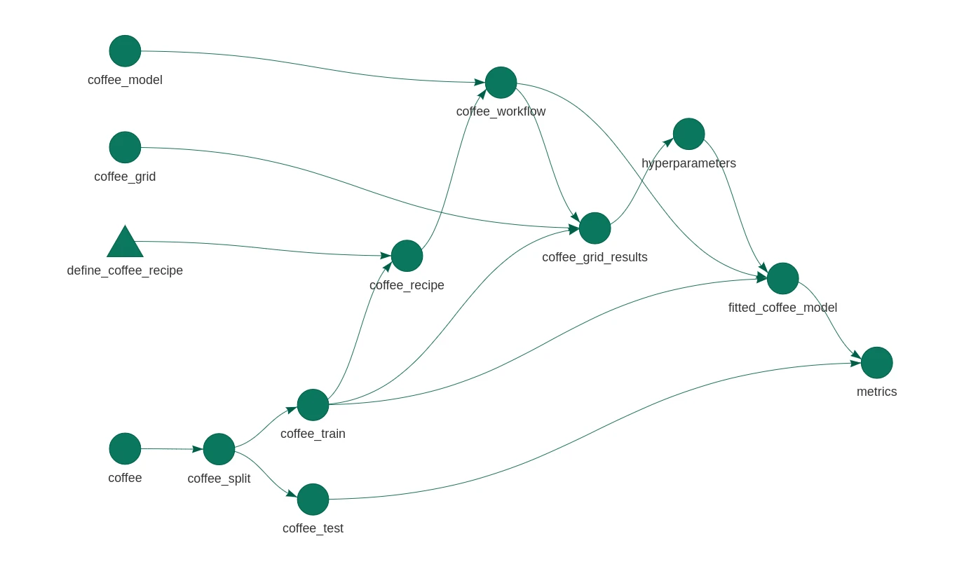
There’s always a need for more tidymodels examples on the Internet. Here’s a simple machine learning model using the recent coffee Tidy Tuesday data set. The plot above gives the approach: I’ll define some preprocessing and a model, optimise some hyperparameters, and fit and evaluate the result. And I’ll piece all of the components together using targets, an experimental alternative to the drake package that I love so much.
As usual, I don’t care too much about the model itself. I’m more interested in the process.
Exploratory data analysis
I’ll start with some token data visualisation. I almost always start exploring new data with the visdat package. It lets me see at a glance the data types, as well as any missing data:
visdat::vis_dat(coffee)
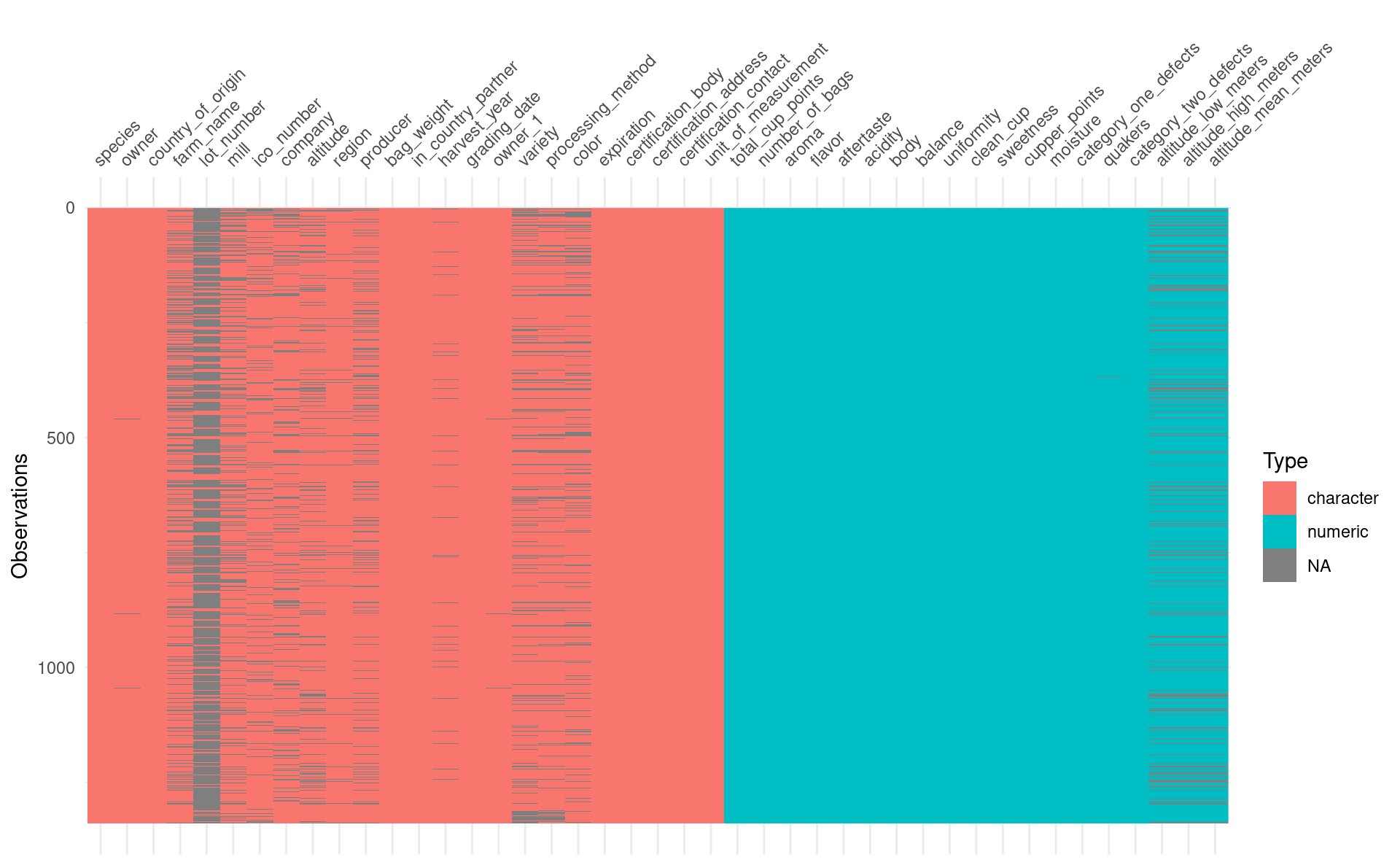
I doubt very much I’ll want to use all of these columns, especially since I only have 1339 rows of data. But some of the columns I do like the look of have missing values, and those will need to be dealt with.
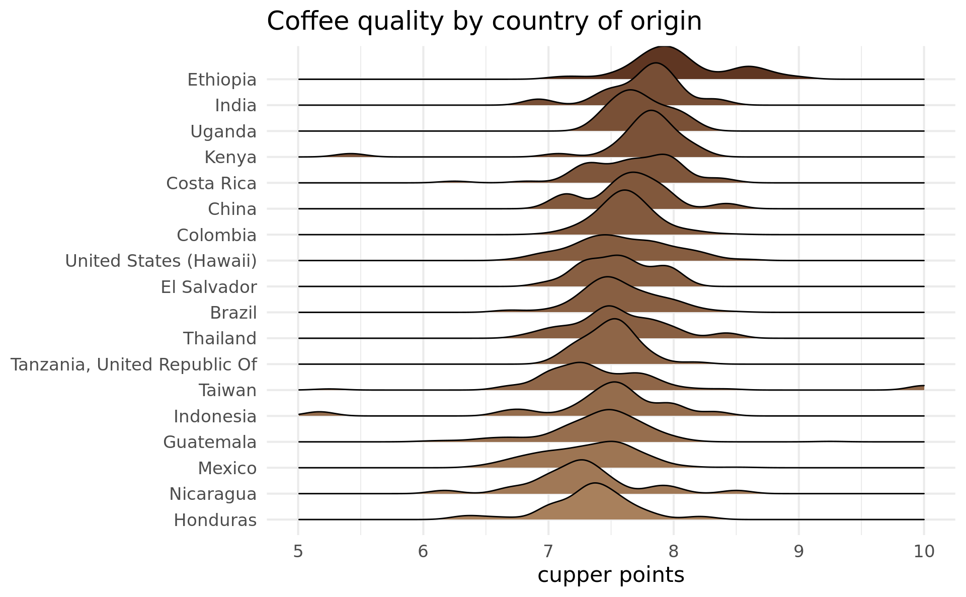
I’ll be looking at cupper_points as a measure of coffee quality, although I’ve seen some analyses on this data use total_cup_points. The cupper_points score ranges from 0 to 10, presumably with 10 being the best. I was curious which countries produce the best coffee, I made a ggplot that makes use of the ggridges package to produce density plots:
coffee %>%
  filter(!is.na(country_of_origin)) %>%
  inner_join(
    coffee %>%
      group_by(country_of_origin) %>%
      summarise(n = n(), average_cupper_points = mean(cupper_points)) %>%
      filter(n / sum(n) > 0.01),
    by = "country_of_origin"
  ) %>%
  ggplot(aes(
    x = cupper_points,
    y = fct_reorder(country_of_origin, average_cupper_points),
    fill = average_cupper_points
  )) +
  ggridges::geom_density_ridges() +
  xlim(5, 10) +
  scale_fill_gradient(low = "#A8805C", high = "#5F3622") +
  ggtitle("Coffee quality by country of origin") +
  xlab("cupper points") +
  ylab(NULL) +
  theme_minimal(base_size = 16, base_family = "Montserrat") +
  theme(legend.position = "none")
Modelling
It’s time to make a model! First I’ll generate an 80/20 train/test split:
set.seed(123)
coffee_split <- initial_split(coffee, prop = 0.8)
coffee_train <- training(coffee_split)
coffee_test <- testing(coffee_split)
The split between test and train is sacred. I start a model by splitting out the test data, and then I forget that it exists until it’s time to evaluate my model. If I introduce any information from coffee_test into coffee_train then I can’t trust my model metrics, since I would have no way of knowing if my model is overfitting. This is called data leakage.
It is very easy to accidentally leak data from test to train. Suppose I have some missing values that I want to impute with the mean. If I impute using the mean of the entire data set, then that’s data leakage. Suppose I scale and centre my numeric variables. I use the mean and variance of the entire data set, then that’s data leakage.
The usual methods of manipulating data often aren’t suitable for preprocessing modelling data. It’s easy enough to centre and scale a variable with mutate(), but data manipulation for machine learning requires tools that respect the split between test and train. That’s what recipes are for.
Preprocessing with recipes
In tidymodels, preprocessing is done with recipes. There’s a particular language for preprocessing with recipes, and it follows a common (and cute) theme. A recipe abstractly defines how to manipulate the data. It is then prepared on a training set, and can be used to bake new data.
Recipes require an understanding of which variables are predictors and which are outcomes (it would make no sense to preprocess the outcome of the test set). Traditionally in R this is done with a formula, like cupper_points ~ flavour + aroma, or cupper_points ~ . if everything as a predictor. Instead, I’m going to use the “role” approach that recipes takes to declare some variables as predictors and cupper_points as an outcome. The rest will be “support” variables, some of which will be used in imputation. I like this approach, since it means that I don’t need to maintain a list of variables to be fed to the fit function. Instead, the fit function will only use the variables with the “predictor” role.
The recipe I’ll use defines the steps below. Just a heads up: I’m not claiming that this is good preprocessing. I haven’t even seen what the impact of this preprocessing is on the resulting model. I’m just using this as an example of some preprocessing steps.
- Sets the roles of every variable in the data. A variable can have more than one role, but here we’ll call everything either “outcome”, “predictor”, or “support”.
tidymodelstreats “outcome” and “predictor” variables specially, but otherwise any string can be a role. - Convert all strings to factors. You read that right.
- Impute
country_of_origin, and thenaltitude_mean_metersusing k-nearest-neighbours with a handful of other variables. - Convert all missing varieties to an “unknown” value.
- Collapse
country_of_origin,processing_methodandvarietylevels so that infrequently occurring values are collapsed to “other”. - Centre and scale all numeric variables.
Many thanks to Julia Silge for helping me define this recipe!
coffee_recipe <- recipe(coffee_train) %>%
  update_role(everything(), new_role = "support") %>%
  update_role(cupper_points, new_role = "outcome") %>%
  update_role(
    variety, processing_method, country_of_origin,
    aroma, flavor, aftertaste, acidity, sweetness, altitude_mean_meters,
    new_role = "predictor"
  ) %>%
  step_string2factor(all_nominal(), -all_outcomes()) %>%
  step_knnimpute(country_of_origin,
                 impute_with = imp_vars(
                 in_country_partner, company, region, farm_name, certification_body
                 )
  ) %>%
  step_knnimpute(altitude_mean_meters,
                 impute_with = imp_vars(
                 in_country_partner, company, region, farm_name, certification_body,
                 country_of_origin
                 )
  ) %>%
  step_unknown(variety, processing_method, new_level = "unknown") %>%
  step_other(country_of_origin, threshold = 0.01) %>%
  step_other(processing_method, variety, threshold = 0.10) %>%
  step_normalize(all_numeric(), -all_outcomes())
coffee_recipe
#> Data Recipe
#>
#> Inputs:
#>
#>       role #variables
#>    outcome          1
#>  predictor          9
#>    support         33
#>
#> Operations:
#>
#> Factor variables from all_nominal(), -all_outcomes()
#> K-nearest neighbor imputation for country_of_origin
#> K-nearest neighbor imputation for altitude_mean_meters
#> Unknown factor level assignment for variety, processing_method
#> Collapsing factor levels for country_of_origin
#> Collapsing factor levels for processing_method, variety
#> Centering and scaling for all_numeric(), -all_outcomes()
I won’t actually need to prep or bake anything here, since that’s all handled for me behind the scenes in the workflow step below. But just to demonstrate, I’ll briefly remember that the test data exists and bake it with this recipe. The baked test data below contains no missing processing_method values. It does, however, contain “unknown” and “Other”.
coffee_recipe %>%
  prep(coffee_train) %>%
  bake(coffee_test) %>%
  count(processing_method)
#> # A tibble: 4 x 2
#>   processing_method     n
#>   <fct>             <int>
#> 1 Natural / Dry        57
#> 2 Washed / Wet        168
#> 3 unknown              28
#> 4 other                14
Model specification
An issue with R’s distributed package ecosystem is that the same variable can have multiple names across different packages. For example, ranger and randomForest are packages used to train random forests, but where ranger uses num.trees to define the number of trees in the forest, randomForest uses ntree. Under tidymodels, these names are standardised to trees. Moreover, the same standard name is used for other models where “number of trees” is a valid concept, such as boosted trees.
Note that I’m setting the hyperparameters with tune(), which means that I expect to fill these values in later. Think of tune() as a placeholder. Apart from trees, the other hyperparameter I’m looking at is mtry. When splitting a branch in a random forest, the algorithm doesn’t have access to all of the variables. It’s only provided with a certain number of randomly chosen variables, and it must select the best one to use to split the data. This number of random variables is mtry.
The “engine” here determines what will be used to fit the model. tidymodels wraps machine learning package, and it has no capacity to train a model by itself. I’m using the ranger package as the engine here, but I could also use the randomForest package.
coffee_model <- rand_forest(
    trees = tune(),
    mtry = tune()
  ) %>%
  set_engine("ranger") %>%
  set_mode("regression")
coffee_model
#> Random Forest Model Specification (regression)
#>
#> Main Arguments:
#>   mtry = tune()
#>   trees = tune()
#>
#> Computational engine: ranger
I haven’t provided any data to the model specification. Just as in Python’s sklearn, in tidymodels models are defined in a separate step to fitting. The above is just a specification for a model.
Workflows
A workflow combines a preprocessing recipe and a model specification. By creating a workflow, all of the preprocessing will be handled for me when fitting the model and when generating new predictions.
coffee_workflow <- workflow() %>%
  add_recipe(coffee_recipe) %>%
  add_model(coffee_model)
coffee_workflow
#> ══ Workflow ═════════════════════════════════════════════════════════════════════════════════════════════════
#> Preprocessor: Recipe
#> Model: rand_forest()
#>
#> ── Preprocessor ─────────────────────────────────────────────────────────────────────────────────────────────
#> 7 Recipe Steps
#>
#> ● step_string2factor()
#> ● step_knnimpute()
#> ● step_knnimpute()
#> ● step_unknown()
#> ● step_other()
#> ● step_other()
#> ● step_normalize()
#>
#> ── Model ────────────────────────────────────────────────────────────────────────────────────────────────────
#> Random Forest Model Specification (regression)
#>
#> Main Arguments:
#>   mtry = tune()
#>   trees = tune()
#>
#> Computational engine: ranger
Hyperparameter tuning
Earlier I set some hyperparameters with tune(), so I’ll need to explore which values I can assign to them. I’ll create a grid of values to explore. Most of these hyperparameters have sensible defaults, but I’ll define my own to be explicit about what I’m doing.
coffee_grid <- expand_grid(mtry = 3:5, trees = seq(500, 1500, by = 200))I’ll use cross-validation on coffee_train to evaluate the performance of each combination of hyperparameters.
set.seed(123)
coffee_folds <- vfold_cv(coffee_train, v = 5)
coffee_folds
#> #  5-fold cross-validation
#> # A tibble: 5 x 2
#>   splits            id
#>   <list>            <chr>
#> 1 <split [857/215]> Fold1
#> 2 <split [857/215]> Fold2
#> 3 <split [858/214]> Fold3
#> 4 <split [858/214]> Fold4
#> 5 <split [858/214]> Fold5
Here’s where I search through the hyperparameter space. With 5 folds and 18 combinations of hyperparameters to explore, R has to train and evaluate 90 models. In general, this sort of tuning takes a while. I could speed this up with parallel processing, but I’m not sure it’s worth the hassle for such a small data set.
coffee_grid_results <- coffee_workflow %>%
  tune_grid(
    resamples = coffee_folds,
    grid = coffee_grid
  )
Now it’s time to see how the models performed! I’ll look at root mean squared error to evaluate this model:
collect_metrics(coffee_grid_results) %>%
    filter(.metric == "rmse") %>%
    arrange(mean) %>%
    head() %>%
    knitr::kable()
| mtry | trees | .metric | .estimator | mean | n | std_err | .config |
|---|---|---|---|---|---|---|---|
| 3 | 1500 | rmse | standard | 0.3127119 | 5 | 0.0565917 | Model06 |
| 3 | 1100 | rmse | standard | 0.3129998 | 5 | 0.0563920 | Model04 |
| 3 | 500 | rmse | standard | 0.3136543 | 5 | 0.0565772 | Model01 |
| 3 | 700 | rmse | standard | 0.3137247 | 5 | 0.0565831 | Model02 |
| 3 | 1300 | rmse | standard | 0.3137998 | 5 | 0.0564674 | Model05 |
| 3 | 900 | rmse | standard | 0.3139521 | 5 | 0.0565038 | Model03 |
tidymodels also comes with some nice auto-plotting functionality for model metrics:
autoplot(coffee_grid_results, metric = "rmse")
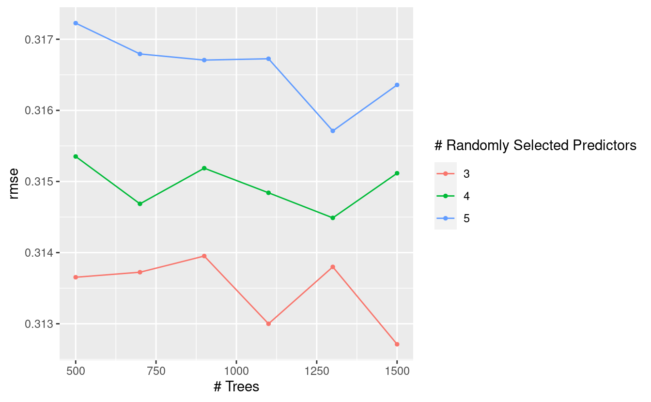
The goal is to minimise RMSE. I can take a look at the hyperparameter combinations that optimise this value:
show_best(coffee_grid_results, metric = "rmse") %>% knitr::kable()
| mtry | trees | .metric | .estimator | mean | n | std_err | .config |
|---|---|---|---|---|---|---|---|
| 3 | 1500 | rmse | standard | 0.3127119 | 5 | 0.0565917 | Model06 |
| 3 | 1100 | rmse | standard | 0.3129998 | 5 | 0.0563920 | Model04 |
| 3 | 500 | rmse | standard | 0.3136543 | 5 | 0.0565772 | Model01 |
| 3 | 700 | rmse | standard | 0.3137247 | 5 | 0.0565831 | Model02 |
| 3 | 1300 | rmse | standard | 0.3137998 | 5 | 0.0564674 | Model05 |
The issue I have here is that 1500 trees is a lot1. When I look at the plot above I can see that 500 trees does pretty well. It may not be the best, but it’s one third as complex.
I think it’s worth cutting back on accuracy a tiny bit if it means simplifying the model a lot. tidymodels contains a function that does just this. I’ll ask for the combination of hyperparameters that minimises the number of trees in the random forest, while not being more than 5% away from the best combination overall:
select_by_pct_loss(coffee_grid_results, metric = "rmse", limit = 5, trees) %>%
  knitr::kable()
| mtry | trees | .metric | .estimator | mean | n | std_err | .config | .best | .loss |
|---|---|---|---|---|---|---|---|---|---|
| 5 | 500 | rmse | standard | 0.3172264 | 5 | 0.0549082 | Model13 | 0.3127119 | 1.443642 |
Model fitting
I can’t fit a model with undefined hyperparameters. I’ll use the above combination to “finalise” the model. Every hyperparameter that I set to “tune” will be set to the result of select_by_pct_loss.
That’s everything I need to fit a model. I have a preprocessing recipe, a model specification, and a nice set of hyperparameters. All that’s left to call is fit:
fitted_coffee_model <- coffee_workflow %>%
  finalize_workflow(
    select_by_pct_loss(coffee_grid_results, metric = "rmse", limit = 5, trees)
  ) %>%
  fit(coffee_train)
Model evaluation
Now that I have a model I can remember that my test set exists. I’ll look at a handful of metrics to see how the model performs. metrics_set(rmse, mae, rsq) is a function that returns a function that compares the true and predicted values. It returns the root mean squared error, mean absolute error, and R squared value.
I’m using some possibly non-idiomatic R code below. metric_set(rmse, mae, rsq) returns a function, so I can immediately call it as a function. This leads to two sets of parameters in brackets right next to each other. There’s nothing wrong with this, but I don’t know if it’s good practice:
fitted_coffee_model %>%
  predict(coffee_test) %>%
  metric_set(rmse, mae, rsq)(coffee_test$cupper_points, .pred)
#> # A tibble: 3 x 3
#>   .metric .estimator .estimate
#>   <chr>   <chr>          <dbl>
#> 1 rmse    standard       0.293
#> 2 mae     standard       0.174
#> 3 rsq     standard       0.506
Targets
There are a lot of steps involved in fitting and evaluating this model, so it would help to have a way to orchestrate the whole process. Normally I would use the drake package for this but Will Landau, its creator and maintainer, has been working on an alternative called targets. This is an experimental package right now, but I thought I’d give it a go for this.
targets will look very familiar to users of drake. Will has laid out some reasons for creating a separate package. drake uses plans, which are R objects. targets takes a similar approach with its pipelines. However, targets requires that the pipeline be defined in a specific _targets.R file. This file can can also set up required functions and objects for the pipeline, and load necessary packages. The requirement is that it ends with a targets pipeline.
I’ve put all of the steps required to fit and evaluate this model into a targets pipeline. The recipe is lengthy, and likely to change often as I refine my preprocessing approach. It’s best to create a function define_coffee_recipe and place it in a file somewhere in my project (probably the R/ directory). I can then source it it within _targets.R. This way, I can change the preprocessing approach without changing the model pipeline. In a complicated project, it would be best to do this for most of the targets, especially the model definition and metrics.
A pipeline consists of a set of tar_targets. The first argument of each is a name for the target, and the second is the command that generates the target’s output. Just as with drake, a pipieline should consist of pure functions: no side-effects, with each target defined only by its inputs and its output. This way, targets can automatically detect the dependencies of each target. A convenient consequence of this is that the order in which the targets are provided is irrelevant, as the package is able to work it out from the dependencies alone.
My _targets.R file with the pipeline is below. Note that the data retrieval step (“coffee”) uses a “never” cue. Like drake, the targets package automatically works out when a step has been invalidated and needs to be rerun. The “never” cue tells targets to never run the “coffee” step unless the result isn’t cached. I can do this because I’m confident that the TidyTuesday data will never change.
library(targets)
source("R/define_coffee_recipe.R")

tar_options(packages = c("tidyverse", "tidymodels"))

tar_pipeline(
  tar_target(
    coffee,
    tidytuesdayR::tt_load(2020, week = 28)$coffee,
    cue = tar_cue("never")
  ),
  tar_target(coffee_split, initial_split(coffee, prop = 0.8)),
  tar_target(coffee_train, training(coffee_split)),
  tar_target(coffee_test, testing(coffee_split)),
  tar_target(coffee_recipe, define_coffee_recipe(coffee_train)),
  tar_target(
    coffee_model,
    rand_forest(
      trees = tune(),
      mtry = tune()
    ) %>% set_engine("ranger") %>% set_mode("regression")
  ),
  tar_target(
    coffee_workflow,
    workflow() %>% add_recipe(coffee_recipe) %>% add_model(coffee_model)
  ),
  tar_target(
    coffee_grid,
    expand_grid(mtry = 3:5, trees = seq(500, 1500, by = 200))
  ),
  tar_target(
    coffee_grid_results,
    coffee_workflow %>%
        tune_grid(resamples = vfold_cv(coffee_train, v = 5), grid = coffee_grid)
  ),
  tar_target(
    hyperparameters,
    select_by_pct_loss(coffee_grid_results, metric = "rmse", limit = 5, trees)
  ),
  tar_target(
    fitted_coffee_model,
    coffee_workflow %>% finalize_workflow(hyperparameters) %>% fit(coffee_train)
  ),
  tar_target(
    metrics,
    fitted_coffee_model %>%
      predict(coffee_test) %>%
      metric_set(rmse, mae, rsq)(coffee_test$cupper_points, .pred)
  )
)
As long as this _targets.R file exists in the working directory the targets package will be able to pick it up and use it. The graph at the top of this page was generated with tar_visnetwork() (no argument necessary). The pipeline can be run with tar_make().
What I love about this orchestration is that I can see where the dependencies are used. I can be sure that the test data isn’t used for preprocessing, or hyperparameter tuning. And it’s just such a pretty plot!
devtools::session_info()
#> ─ Session info ───────────────────────────────────────────────────────────────
#>  setting  value
#>  version  R version 4.0.0 (2020-04-24)
#>  os       Ubuntu 20.04 LTS
#>  system   x86_64, linux-gnu
#>  ui       X11
#>  language en_AU:en
#>  collate  en_AU.UTF-8
#>  ctype    en_AU.UTF-8
#>  tz       Australia/Melbourne
#>  date     2020-07-27
#>
#> ─ Packages ───────────────────────────────────────────────────────────────────
#>  package     * version    date       lib source
#>  assertthat    0.2.1      2019-03-21 [1] CRAN (R 4.0.0)
#>  backports     1.1.8      2020-06-17 [1] CRAN (R 4.0.0)
#>  blob          1.2.1      2020-01-20 [1] CRAN (R 4.0.0)
#>  broom       * 0.7.0      2020-07-09 [1] CRAN (R 4.0.0)
#>  callr         3.4.3      2020-03-28 [1] CRAN (R 4.0.0)
#>  cellranger    1.1.0      2016-07-27 [1] CRAN (R 4.0.0)
#>  class         7.3-17     2020-04-26 [4] CRAN (R 4.0.0)
#>  cli           2.0.2      2020-02-28 [1] CRAN (R 4.0.0)
#>  codetools     0.2-16     2018-12-24 [4] CRAN (R 4.0.0)
#>  colorspace    1.4-1      2019-03-18 [1] CRAN (R 4.0.0)
#>  crayon        1.3.4      2017-09-16 [1] CRAN (R 4.0.0)
#>  data.table    1.13.0     2020-07-24 [1] CRAN (R 4.0.0)
#>  DBI           1.1.0      2019-12-15 [1] CRAN (R 4.0.0)
#>  dbplyr        1.4.4      2020-05-27 [1] CRAN (R 4.0.0)
#>  desc          1.2.0      2018-05-01 [1] CRAN (R 4.0.0)
#>  devtools      2.3.0      2020-04-10 [1] CRAN (R 4.0.0)
#>  dials       * 0.0.8      2020-07-08 [1] CRAN (R 4.0.0)
#>  DiceDesign    1.8-1      2019-07-31 [1] CRAN (R 4.0.0)
#>  digest        0.6.25     2020-02-23 [1] CRAN (R 4.0.0)
#>  downlit       0.0.0.9000 2020-07-25 [1] Github (r-lib/downlit@ed969d0)
#>  dplyr       * 1.0.0      2020-05-29 [1] CRAN (R 4.0.0)
#>  ellipsis      0.3.1      2020-05-15 [1] CRAN (R 4.0.0)
#>  evaluate      0.14       2019-05-28 [1] CRAN (R 4.0.0)
#>  fansi         0.4.1      2020-01-08 [1] CRAN (R 4.0.0)
#>  farver        2.0.3      2020-01-16 [1] CRAN (R 4.0.0)
#>  forcats     * 0.5.0      2020-03-01 [1] CRAN (R 4.0.0)
#>  foreach       1.5.0      2020-03-30 [1] CRAN (R 4.0.0)
#>  fs            1.4.2      2020-06-30 [1] CRAN (R 4.0.0)
#>  furrr         0.1.0      2018-05-16 [1] CRAN (R 4.0.0)
#>  future        1.17.0     2020-04-18 [1] CRAN (R 4.0.0)
#>  generics      0.0.2      2018-11-29 [1] CRAN (R 4.0.0)
#>  ggplot2     * 3.3.2.9000 2020-07-10 [1] Github (tidyverse/ggplot2@a11e098)
#>  ggridges      0.5.2      2020-01-12 [1] CRAN (R 4.0.0)
#>  globals       0.12.5     2019-12-07 [1] CRAN (R 4.0.0)
#>  glue          1.4.1      2020-05-13 [1] CRAN (R 4.0.0)
#>  gower         0.2.2      2020-06-23 [1] CRAN (R 4.0.0)
#>  GPfit         1.0-8      2019-02-08 [1] CRAN (R 4.0.0)
#>  gtable        0.3.0      2019-03-25 [1] CRAN (R 4.0.0)
#>  hardhat       0.1.4      2020-07-02 [1] CRAN (R 4.0.0)
#>  haven         2.2.0      2019-11-08 [1] CRAN (R 4.0.0)
#>  highr         0.8        2019-03-20 [1] CRAN (R 4.0.0)
#>  hms           0.5.3      2020-01-08 [1] CRAN (R 4.0.0)
#>  htmltools     0.5.0      2020-06-16 [1] CRAN (R 4.0.0)
#>  httr          1.4.2      2020-07-20 [1] CRAN (R 4.0.0)
#>  hugodown      0.0.0.9000 2020-07-25 [1] Github (r-lib/hugodown@3980496)
#>  igraph        1.2.5      2020-03-19 [1] CRAN (R 4.0.0)
#>  infer       * 0.5.3      2020-07-14 [1] CRAN (R 4.0.0)
#>  ipred         0.9-9      2019-04-28 [1] CRAN (R 4.0.0)
#>  iterators     1.0.12     2019-07-26 [1] CRAN (R 4.0.0)
#>  jsonlite      1.7.0      2020-06-25 [1] CRAN (R 4.0.0)
#>  knitr         1.29       2020-06-23 [1] CRAN (R 4.0.0)
#>  labeling      0.3        2014-08-23 [1] CRAN (R 4.0.0)
#>  lattice       0.20-41    2020-04-02 [4] CRAN (R 4.0.0)
#>  lava          1.6.7      2020-03-05 [1] CRAN (R 4.0.0)
#>  lhs           1.0.2      2020-04-13 [1] CRAN (R 4.0.0)
#>  lifecycle     0.2.0      2020-03-06 [1] CRAN (R 4.0.0)
#>  listenv       0.8.0      2019-12-05 [1] CRAN (R 4.0.0)
#>  lubridate     1.7.8      2020-04-06 [1] CRAN (R 4.0.0)
#>  magrittr      1.5        2014-11-22 [1] CRAN (R 4.0.0)
#>  MASS          7.3-51.6   2020-04-26 [4] CRAN (R 4.0.0)
#>  Matrix        1.2-18     2019-11-27 [4] CRAN (R 4.0.0)
#>  memoise       1.1.0.9000 2020-05-09 [1] Github (hadley/memoise@4aefd9f)
#>  modeldata   * 0.0.2      2020-06-22 [1] CRAN (R 4.0.0)
#>  modelr        0.1.6      2020-02-22 [1] CRAN (R 4.0.0)
#>  munsell       0.5.0      2018-06-12 [1] CRAN (R 4.0.0)
#>  nnet          7.3-14     2020-04-26 [4] CRAN (R 4.0.0)
#>  parsnip     * 0.1.2      2020-07-03 [1] CRAN (R 4.0.0)
#>  pillar        1.4.6      2020-07-10 [1] CRAN (R 4.0.0)
#>  pkgbuild      1.0.8      2020-05-07 [1] CRAN (R 4.0.0)
#>  pkgconfig     2.0.3      2019-09-22 [1] CRAN (R 4.0.0)
#>  pkgload       1.1.0      2020-05-29 [1] CRAN (R 4.0.0)
#>  plyr          1.8.6      2020-03-03 [1] CRAN (R 4.0.0)
#>  prettyunits   1.1.1      2020-01-24 [1] CRAN (R 4.0.0)
#>  pROC          1.16.2     2020-03-19 [1] CRAN (R 4.0.0)
#>  processx      3.4.3      2020-07-05 [1] CRAN (R 4.0.0)
#>  prodlim       2019.11.13 2019-11-17 [1] CRAN (R 4.0.0)
#>  ps            1.3.3      2020-05-08 [1] CRAN (R 4.0.0)
#>  purrr       * 0.3.4      2020-04-17 [1] CRAN (R 4.0.0)
#>  R6            2.4.1      2019-11-12 [1] CRAN (R 4.0.0)
#>  ranger        0.12.1     2020-01-10 [1] CRAN (R 4.0.0)
#>  Rcpp          1.0.5      2020-07-06 [1] CRAN (R 4.0.0)
#>  readr       * 1.3.1      2018-12-21 [1] CRAN (R 4.0.0)
#>  readxl        1.3.1      2019-03-13 [1] CRAN (R 4.0.0)
#>  recipes     * 0.1.13     2020-06-23 [1] CRAN (R 4.0.0)
#>  remotes       2.1.1      2020-02-15 [1] CRAN (R 4.0.0)
#>  reprex        0.3.0      2019-05-16 [1] CRAN (R 4.0.0)
#>  rlang         0.4.7      2020-07-09 [1] CRAN (R 4.0.0)
#>  rmarkdown     2.3.3      2020-07-25 [1] Github (rstudio/rmarkdown@204aa41)
#>  rpart         4.1-15     2019-04-12 [4] CRAN (R 4.0.0)
#>  rprojroot     1.3-2      2018-01-03 [1] CRAN (R 4.0.0)
#>  rsample     * 0.0.7      2020-06-04 [1] CRAN (R 4.0.0)
#>  rstudioapi    0.11       2020-02-07 [1] CRAN (R 4.0.0)
#>  rvest         0.3.5      2019-11-08 [1] CRAN (R 4.0.0)
#>  scales      * 1.1.1      2020-05-11 [1] CRAN (R 4.0.0)
#>  sessioninfo   1.1.1      2018-11-05 [1] CRAN (R 4.0.0)
#>  stringi       1.4.6      2020-02-17 [1] CRAN (R 4.0.0)
#>  stringr     * 1.4.0      2019-02-10 [1] CRAN (R 4.0.0)
#>  survival      3.1-12     2020-04-10 [4] CRAN (R 4.0.0)
#>  targets     * 0.0.0.9000 2020-07-25 [1] Github (wlandau/targets@1455610)
#>  testthat      2.3.2      2020-03-02 [1] CRAN (R 4.0.0)
#>  tibble      * 3.0.3      2020-07-10 [1] CRAN (R 4.0.0)
#>  tidymodels  * 0.1.1      2020-07-14 [1] CRAN (R 4.0.0)
#>  tidyr       * 1.1.0      2020-05-20 [1] CRAN (R 4.0.0)
#>  tidyselect    1.1.0      2020-05-11 [1] CRAN (R 4.0.0)
#>  tidyverse   * 1.3.0      2019-11-21 [1] CRAN (R 4.0.0)
#>  timeDate      3043.102   2018-02-21 [1] CRAN (R 4.0.0)
#>  tune        * 0.1.1      2020-07-08 [1] CRAN (R 4.0.0)
#>  usethis       1.6.1      2020-04-29 [1] CRAN (R 4.0.0)
#>  utf8          1.1.4      2018-05-24 [1] CRAN (R 4.0.0)
#>  vctrs         0.3.2      2020-07-15 [1] CRAN (R 4.0.0)
#>  visdat        0.5.3      2019-02-15 [1] CRAN (R 4.0.0)
#>  withr         2.2.0      2020-04-20 [1] CRAN (R 4.0.0)
#>  workflows   * 0.1.2      2020-07-07 [1] CRAN (R 4.0.0)
#>  xfun          0.16       2020-07-24 [1] CRAN (R 4.0.0)
#>  xml2          1.3.2      2020-04-23 [1] CRAN (R 4.0.0)
#>  yaml          2.2.1      2020-02-01 [1] CRAN (R 4.0.0)
#>  yardstick   * 0.0.7      2020-07-13 [1] CRAN (R 4.0.0)
#>
#> [1] /home/mdneuzerling/R/x86_64-pc-linux-gnu-library/4.0
#> [2] /usr/local/lib/R/site-library
#> [3] /usr/lib/R/site-library
#> [4] /usr/lib/R/library
Adding more trees to a random forest doesn’t make the model overfit, or have any other detriment on model performance. But additional trees do carry a computational cost, in both model training and prediction. It’s good to keep the number as low as possible without harming model performance.↩︎